Linear regression is one of the most popular and simplest machine learning models that capture the relationship between two or more features. The objective of linear regression is to draw a line of best fit for performing predictions and inferences.

NOTE

Linear regression is also a classic statistical model, but this guide will treat linear regression as a machine learning model. This means that topics such as p-values, inferences and distributions will not be covered.

Simple example of linear regression by hand

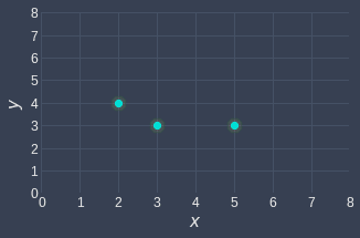
Suppose we have the following data points:

Let's start simple and build a linear regression model that goes through the origin. The objective therefore is to find a line of best fit that passes the origin.

What are cost functions?

In order to judge which lines fit better, we need a way to quantify the lines' performance. For example, consider the following two lines:

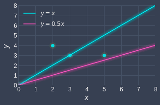
Intuitively, we can tell that the blue line fits our data points better than the red line because the blue line is relatively closer to the data points.

By convention in machine learning, the performance of a model is based on how inaccurate it is, rather than how accurate it is. For linear regression, this means that we want to measure how far off a model's fitted points are from the true data points. A line that is only off by a small amount implies that the line does an excellent job at modeling the data points.

Now, instead of talking about the performance of a model in abstract terms, we want to come up with a mathematical expression to quantify this notion of how off the model is. In machine learning, this expression is known as the cost function.

Cost functions play a central role in machine learning, and they capture how inaccurate a model is. A high value for the cost function means that the model is performing badly, while a low value means that the model is performing well. The objective then is to find a line that minimizes the cost function.

Formulating the cost function

For linear regression, the cost function is easy to derive - all we have to do is to compute the distances between our data points and the corresponding points on the fitted line, and then sum them up. Using our previous example, this means that we need to compute the sum of the red dashed lines as well as the sum of the blue dashed lines:

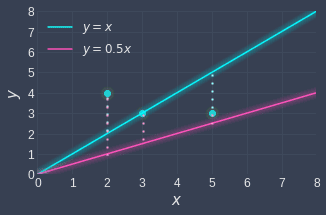
Mathematically, this involves computing a metric called the sum of squared errors (SSE):

$$J=\frac{1}{2}\sum^m_{i=1}\left(y_i-\hat{y}_i\right)^2$$

Where:

$J$ is the cost function, which represents the quantity we want to minimize
$m$ is the number of data points ($3$ in this case)
$y_i$ is the $y$ value of the $i$-th data point (e.g. $y_1=4$)
$\hat{y}_i$ is the fitted $y$ value of the $i$-th data point (e.g. $\hat{y}_1=1$ for the red fitted line)

Formulating the cost function is only half the battle won - we now need to compute the parameters of the model that minimize the cost function.

NOTE

We often add a $\frac{1}{2}$ term at the front of the sum of squared errors (SSE) for convenience when computing the derivativelink.

Computing the cost function

Now that we've covered why the cost function is written the way that it is, we'll run through a quick example of actually computing the cost function. Recall that our example was as follows:

As a refresher, here's the cost function again:

$$J=\frac{1}{2}\sum^m_{i=1}\left(y_i-\hat{y}_i\right)^2$$

To compute the respective cost for the blue and red lines:

$$\begin{align} J_{\mathrm{blue}}&=\frac{1}{2} \left[ (4-2)^2+(3-3)^2+(3-5)^2\right]=4 \\ J_{\mathrm{red}}&=\frac{1}{2} \left[ (4-1)^2+(3-1.5)^2+(3-2.5)^2\right]=5.75 \\ \end{align}$$

The fact that $J_{\mathrm{blue}}\lt{J_{\mathrm{red}}}$ confirms our intuition that the blue line fits the data points more accurately. Remember, the cost function represents how off a model is, so the lower the cost function, the better the model is.

Examining the cost function

Purpose of squaring the difference

Notice how we have the squared term $(y_i−\hat{y}_i)^2$ in the cost function, which you might find strange since $y_i−\hat{y}_i$ already captures the inaccuracy of our model.

The reason for this is that whether our data points are above or below the fitted line should not matter - we are only concerned about how off we are. Without the square, we would end up having positive and negative differences:

when the estimated value ($\hat{y}_i$) is smaller than the true value ($y_i$), then the difference $y_i-\hat{y}_i$ will be positive.
when the estimated value is larger than the true value, then the difference $y_i−\hat{y}_i$ will be negative.

If we were to compute the sum of these differences, the positive and negative differences will cancel each other out, thereby reducing the total error. For example, suppose we have the following scenario:

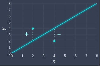
If we did not include the square term here, then the error terms would simply cancel each other out, and hence the cost function will equal 0, indicating a perfect fit! Clearly, this isn't correct since the line does not go through all the points. To avoid traps like this, we must square the differences.

Squaring versus taking absolute value

You may be wondering why we take the square instead of taking the absolute value. After all, taking the absolute value $|y-\hat{y}_i|$ does remove negative differences. You might also argue that taking the absolute value is a better measure of error because squaring the differences inflates the cost function.

You are right - but absolute values don't work well with derivatives, and this becomes a problem later on when we compute the derivative of the cost function.

It also does not matter if the cost value gets inflated due to the squaring because:

we are typically concerned with finding the parameters that minimize the error, that is, the final value of the cost function is less important.
we can still objectively compare the performance of two linear regression models as long as we use the same cost function.

Finding the line of best fit

In the previous sectionlink, we compared the performance of two models by computing their cost function. We are now ready to tackle the more interesting challenge of actually finding the line of best fit, which involves deriving the optimal parameters.

In our example, we are only interested in finding the line of best fit that goes through the origin, so the parameter that we want to find is just the slope. A line that passes through the origin will always be of the following form:

$$\begin{equation}\label{eq:zYSDxCiavPk59oFGtj2} \hat{y}=\theta{x} \end{equation}$$

Here, $\theta$ represents the slope of the line, and it is the parameter that we want to optimize.

Recall that the cost function we wish to minimize is the sum of squared errors (SSE):

$$\begin{equation}\label{eq:anVKD8bMNp4iqy5Q1iU} J=\frac{1}{2}\sum^m_{i=1}\left(y_i-\hat{y}_i\right)^2 \end{equation}$$

Substituting \eqref{eq:zYSDxCiavPk59oFGtj2} into \eqref{eq:anVKD8bMNp4iqy5Q1iU} gives:

$$\begin{equation}\label{eq:h5bOO2Hxf5pgL7k0nL8} J(\theta)=\frac{1}{2}\sum^m_{i=1}\left(y_i-\theta{x_i} \right)^2 \end{equation}$$

Notice how the cost function $J$ has been rewritten as $J(\theta)$ to indicate that our cost function is only dependent on $\theta$ since our data points $(x_i,y_i)$ are fixed. Let's substitute our data points into \eqref{eq:h5bOO2Hxf5pgL7k0nL8}:

$$\begin{equation}\label{eq:kvzXyAOGVpI7q80e0TR} J(\theta)=\frac{1}{2} \Big[\left(4-2\theta \right)^2+ \left(3-3\theta \right)^2+ \left(3-5\theta \right)^2 \Big] \end{equation}$$

This is exactly what we've done in the previous section, but the only difference is that instead of computing the cost function of a defined line (e.g. $y=2x$), we are now computing the cost function of a general line $y=\theta x$.

Simplifying \eqref{eq:kvzXyAOGVpI7q80e0TR} gives us the following:

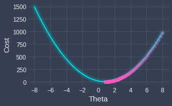
$$\begin{equation}\label{eq:LlEioAlcvGYL7JLFzbt} J(\theta)=17-32\theta+19\theta^2 \end{equation}$$

Notice how our cost function $J(\theta)$ is simply a parabola, which visually looks like the following:

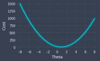
We can see that the cost is minimized when $\theta\approx1$. Instead of eyeballing, we can compute the actual $\theta$ value that minimizes the cost function in one of the following ways:

analytical approach - we use old-school calculus; take the first derivative and equate it to zero. This approach gives you exact answers, but for complex models, computing the derivative is time-consuming and tedious.
numerical approach - we rely on algorithms designed to find the optimal solution. Although this approach may not always return the optimal solution, it can handle complex models far better than the analytical approach.

In statistics, we normally use the analytical approach, whereas in machine learning, the numerical approach is more commonplace. Since this is a tutorial about linear regression in the context of machine learning, we will use the numerical approach of applying an algorithm called gradient descent.

Minimizing the cost function using gradient descent

What is gradient descent?

Gradient descent is an iterative algorithm that aims to find inputs that minimize a particular function. Our goal is to apply gradient descent to compute the parameter $\theta$ that minimizes the cost function.

We won't explain how gradient descent works here as we already have a comprehensive guide on gradient descent, so please check that out first and come back here.

* * *

The update rule of gradient descent for our cost function $J(\theta)$ is as follows:

$$\begin{equation}\label{eq:x5SRHn36Ab9lCPXiVmp} \theta^{(i+1)}=\theta^{(i)}-\alpha\frac{dJ}{d\theta} \end{equation}$$

Where:

$\theta^{(i)}$ is the value of the parameter $\theta$ at iteration $i$
$\theta^{(i+1)}$ is the updated value
$\alpha$ is the learning rate (e.g. $\alpha=0.001$)

The gradient is computed by taking the derivative of our cost function \eqref{eq:LlEioAlcvGYL7JLFzbt} with respect to $\theta$, that is:

$$\begin{equation}\label{eq:gSaBUaRTj7NBYwctdYL} \frac{dJ}{d\theta}=-32+38\theta \end{equation}$$

Substituting \eqref{eq:gSaBUaRTj7NBYwctdYL} into \eqref{eq:x5SRHn36Ab9lCPXiVmp} gives:

$$\begin{equation}\label{eq:u4vgm7tGZEpUsKaOvlH} \begin{aligned} \theta^{(i+1)}&=\theta^{(i)}-\alpha(-32+38\theta^{(i)})\\ \end{aligned} \end{equation}$$

The three hyper-parameter values that we set are:

learning rate - let's say $\alpha=0.001$.
the starting value of $\theta$ - let's say $\theta^{(0)}=8$.
some terminating condition - let's say $150$ iterations.

Substituting $\alpha=0.001$ into \eqref{eq:u4vgm7tGZEpUsKaOvlH}, and then simplifying gives:

$$\begin{equation}\label{eq:EEz4k84fFf9869CQD26} \theta^{(i+1)}=0.962\theta^{(i)}+0.032 \end{equation}$$

When we apply gradient descent, we end up with the following result:

As we can see, we start from $\theta=8$ and then make our way downwards to the minimum of the cost function at each iteration of the gradient descent. The final result of gradient descent is as follows:

$$\begin{align*} \theta^{(150)}&\approx0.86\\ J^{(150)}&\approx3.54 \end{align*}$$

Here, the superscript $(150)$ indicates the value after $150$ iterations. We now know that the optimal $\theta$ is around $0.86$, we can write the line of best fit like so:

$$y=0.86x$$

Great, let's visualize this line to see just how well it fits the actual data points:

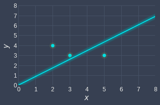
The line $y=0.86x$ is the line of best fit - no other line (that passes through the origin) can top its accuracy.

Linear regression model with an intercept term

In the previous example, we imposed the constraint that the line of best fit must go through the origin. This allowed us to ignore the intercept term and construct a model that is dependent on a single parameter $\theta$, which represented the slope.

In this section, we will build a slightly more complex model with two parameters:

$$\begin{equation}\label{eq:zpvchcZ3vcMmStClVAx} \hat{y}=\theta_0+\theta_1x \end{equation}$$

Once again, consider the same data points:

Recall that the general form of the cost function was as follows:

$$\begin{equation}\label{eq:MfHboadboJPfu2fcuat} J=\frac{1}{2}\sum^m_{i=1}\left(y_i-\hat{y}_i\right)^2\\ \end{equation}$$

Substituting \eqref{eq:zpvchcZ3vcMmStClVAx} into \eqref{eq:MfHboadboJPfu2fcuat} gives:

$$\begin{equation}\label{eq:i3Z9fnJGJz2GFTcPzr5} J(\theta_0,\theta_1)=\frac{1}{2}\sum^3_{i=1}\Big(y_i-(\theta_0+\theta_1x_i)\Big)^2 \end{equation}$$

Notice how the cost function is now dependent on two parameters $\theta_0$ and $\theta_1$. Substituting in the data points $(x_i,y_i)$ and simplifying \eqref{eq:i3Z9fnJGJz2GFTcPzr5} gives:

$$\begin{equation}\label{eq:dI0gtacPjvKWdiJX5CL} J(\theta_0,\theta_1)=\frac{1}{2}(3x^2+20xy-20x+37y^2-64y+34) \end{equation}$$

Visually, our cost function looks like this:

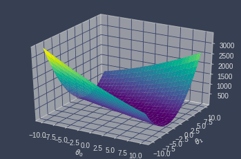
Our goal is to find the $(\theta_0,\theta_1)$ pair that minimizes this function using gradient descent once again.

In the case of two parameters, the update functions for gradient descent involve partial derivatives:

$$\begin{equation}\label{eq:iHpD8WG5LrsTdK7FMte} \begin{aligned} \theta_0&=\theta_0-\alpha\frac{dJ}{d\theta_0}\\ \theta_1&=\theta_1-\alpha\frac{dJ}{d\theta_1}\\ \end{aligned} \end{equation}$$

To derive the general update functions in terms of $\theta_0$ and $\theta_1$, let's stick with \eqref{eq:i3Z9fnJGJz2GFTcPzr5} instead of \eqref{eq:dI0gtacPjvKWdiJX5CL}. Let's begin by taking the partial derivative of $J$ with respect to $\theta_0$:

$$\begin{equation}\label{eq:LGvsD5kvcn6Nnsumojd} \begin{aligned}[b] \frac{\partial{J}}{\partial{\theta_0}}&= \frac{\partial}{\partial{\theta_0}} \Big( \frac{1}{2}\sum^3_{i=1}\Big(y_i-(\theta_0+\theta_1x_i)\Big)^2 \Big)\\ &= \frac{1}{2}\sum^3_{i=1}\frac{\partial}{\partial{\theta_0}}\Big(y_i-(\theta_0+\theta_1x_i)\Big)^2\\ &=\sum^3_{i=1}\Big(y_i-(\theta_0+\theta_1x_i)\Big)(-1)\\ &=\sum^3_{i=1}\Big(-y_i+(\theta_0+\theta_1x_i)\Big)\\ \end{aligned} \end{equation}$$

Similarly, the partial derivative of $J$ with respect to $\theta_1$ would be as follows:

$$\begin{align*} \frac{\partial{J}}{\partial{\theta_1}}&= \sum^3_{i=1}\Big(-x_iy_i+x_i(\theta_0+\theta_1x_i)\Big)\\ \end{align*}$$

With the partial derivatives now derived, let's substitute them into our update functions \eqref{eq:iHpD8WG5LrsTdK7FMte}:

$$\begin{align*} \theta_0&=\theta_0-\alpha\frac{dJ}{d\theta_0}\\ &=\theta_0-\alpha \sum^m_{i=1}\Big(y_i-(\theta_0+\theta_1x_i)\Big) \end{align*}$$

Similarly, the update function for $\theta_1$ is:

$$\begin{align*} \theta_1&=\theta_1-\alpha\frac{dJ}{d\theta_1}\\ &=\theta_1-\alpha \sum^m_{i=1}\Big(y_i+x_i(\theta_0+\theta_1x_i)\Big) \end{align*}$$

Now, suppose we set the following three hyper-parameter values for gradient descent:

learning rate $\alpha=0.001$.
starting point $(\theta_0,\theta_1)=(8,8)$.
number of iterations to $1000$.

The following contour plot illustrates the change in our position as we iteratively descend the function:

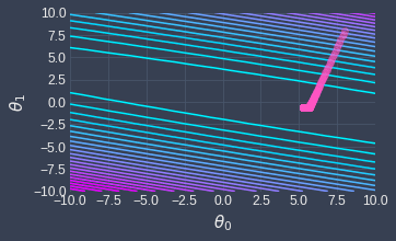
The light blue lines represent low values of the cost function while the purple lines indicate high values. We can see that, at each step of gradient descent, we land at a point that gives us a lower value of the cost function.

We can confirm this by visualizing how the cost function changes over the iterations:

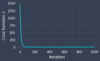
The final output of gradient descent is the optimal values of $\theta_0$ and $\theta_1$ that minimize the cost function $J$:

$$\begin{align*} \theta_0&\approx2.86\\ \theta_1&\approx0.09 \end{align*}$$

Therefore, the line of best fit is as follows:

$$\begin{equation}\label{eq:n9xbxBWx2qRy5JBE7pw} \hat{y}=2.86+0.09x \end{equation}$$

Graphically, this looks like the following:

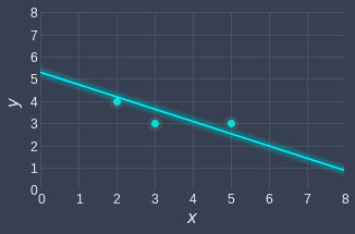
This looks much better than the slope-only model ($y=0.86x$) that we fit earlier:

In fact, we can compare the optimal cost function values to know which model performs better:

$$\begin{align*} \text{Cost with intercept}\approx0.18\\ \text{Cost without intercept}\approx3.54 \end{align*}$$

We see that the final cost with the intercept term is much less than that without the intercept!

Closing thoughts

Linear regression is one of the simplest machine learning models that is widely used in practice. The cost function for linear regression is the sum of squared errors (SSE), and we typically use an optimization technique called gradient descent to find the parameters that minimize the cost function.

We only covered the basics of linear regression here, but there are far more topics to discuss such as:

issues with under-fitting and over-fitting.
how to pick a suitable regression formula. We only tried two formulas here (one without the intercept and one with the intercept), but are there other regression lines that fit the dataset better?

I will write another comprehensive guide that covers these aspects of linear regression soon, so please join our newsletteropen_in_new to be notified when I publish.

Did you have any questions while reading this article? Please let me know in the comments for any questions or feedback, or send me an email at isshin@skytowner.com.

Published by Isshin Inada

Edited by 0 others

Did you find this page useful?

thumb_up

thumb_down

Comment

Citation

Ask a question or leave a feedback...

thumb_up

thumb_down

chat_bubble_outline

settings

Enjoy our search

Hit / to insta-search docs and recipes!