In essence, gradient descent is an iterative algorithm used to determine the value of inputs that minimize a particular function. In the context of machine learning, gradient descent is often used to minimize the cost function.

Simple example of gradient descent

Consider the function $f(x)=(x-1)^2$:

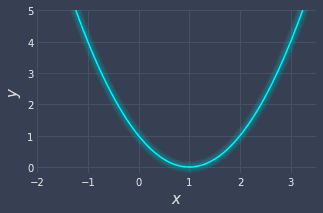
Our goal is to determine the value of $x$ that minimizes this function using gradient descent. Visually, we can see that the minimum occurs at $x=1$. This visual approach only works when the function is simple. More often than not, the functions you want to minimize are far more complex with large number of inputs.

The gradient descent algorithm begins by selecting a point of departure - say at $x=3$:

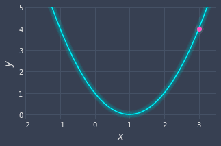
Clearly, $x=3$ is not the optimal value that minimizes the function. The question that the gradient descent algorithm repetitively asks is simple - which direction do I head towards to minimize the function. In other words, should I go rightwards and select values like $x=4$, or should I go leftwards and select values like $x=2$? Visually once again, we can see that $ x=2$ does a far better job in minimizing our function than $x=4$, so then we should take a step to the left as it would take us closer to the minimum of the function.

Instead of relying on visuals to decide which direction to head towards, we could instead make good use of the gradient. The gradient, or the slope, tells us which direction to head towards. If the slope is positive, then we need to head leftwards, and if the slope is negative, then we need to head rightwards.

For example, at $x=3$, we have a positive slope:

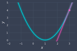
Since the slope is positive, we need to head to the left in order to minimize our function $f(x)$.

Note that if we had started at $x=-1$, the slope would be negative:

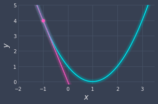
Since the slope is negative, we would have to head rightwards in this case to minimize $f(x)$.

Using basic calculus, we know that the gradient of $f(x)$ is as follows:

$$f'(x)=2x-2$$

At $x=3$, we have a gradient of $4$:

$$\begin{align*} f'(3)&=2(3)-2\\ &=4 \end{align*}$$

Gradient descent involves taking a step to the left if the gradient is positive, while taking a step to the right if the gradient is negative. Mathematically, a step would take us from the current value of $x$ to a new value of $x^*$, which is supposedly better because the function value may be smaller, that is, $f(x^*)\lt{f(x)}$. A simple version of gradient descent iteratively applies the following update formula to compute a new value of $x$:

$$\begin{equation}\label{eq:UhevCzeNbdSxRO09OXD} x^{(i+1)}=x^{(i)}-f'(x^{(i)}) \end{equation}$$

Here, $x^{(i)}$ is the current value of $x$ at iteration $i$, while $x^{(i+1)}$ is the updated value of $x$.

Let's use \eqref{eq:UhevCzeNbdSxRO09OXD} to update our value of $x$ from the starting point $x^{(0)}$ to $x^{(1)}$:

$$\begin{align*} x^{(1)}&=x^{(0)}-f'(3)\\ &=3-4\\ &=-1 \end{align*}$$

This tells us that the new value of $x$ is $-1$. Let's check whether the new value of $x$ is better:

$$\begin{align*} f(-1)&=(-1-1)^2\\ &=4 \end{align*}$$

Let's plot our new position $(-1,4)$ to see whether there was any improvement:

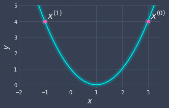
Unfortunately, our new value of $x$ did not decrease our function value. We did move leftwards, which is the correct direction, but the problem is that the step we took was too big. We overstepped and missed the minimum entirely!

In order to adjust the step size, gradient descent uses a parameter known as the learning rate $\alpha$:

$$x^{(i+1)}=x^{(i)}-\alpha\cdot{f'(x^{(i)})}$$

The learning rate $\alpha$ is a numerical value (e.g. $0.01$) that tells us how big of a step we should take at each iteration of the gradient descent. There is a tradeoff when selecting $\alpha$. A small value of $\alpha$ means that we are taking a small step. While this does prevent overshooting like in the case we just encountered, this would involve more iterations to get to the minimum.

On the other hand, a large value for $\alpha$ involves taking large steps to get to the minimum faster, but there is a high risk of overshooting - our step might be so large that we might miss the minimum and end up at a value of $x$ that may even be further away from the optimal point than we started!

As an example, let's set a learning rate of $\alpha=0.1$ to perform an update:

$$\begin{align*} x^{(1)}&=x^{(0)}-\alpha\times{f'(x^{(0)})}\\ &=3-0.1\times{f'(3)}\\ &=3-0.1\times4\\ &=2.6 \end{align*}$$

Let's plot the point at $x=2.6$:

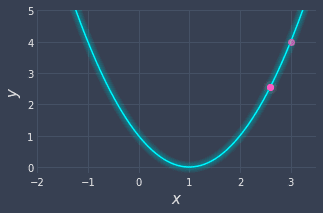
We can see that the point is closer to the minimum! Now, we just need to iteratively repeat this process:

$$\begin{align*} x^{(2)} &=x^{(1)}-\alpha\cdot{f'(x^{(1)})}\\ &=2.6-0.1\cdot{f'(2.6)}\\ &=2.28 \end{align*}$$

Visually, the updated data point looks like the following:

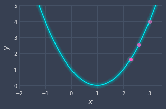
Great, our point is getting closer and closer to the minimum!

We just need to repetitively apply equation \eqref{eq:UhevCzeNbdSxRO09OXD} until one of the following terminating conditions is met:

the iteration count reaches a predefined limit (e.g. 1000 iterations at most)
further iterations do not minimize the function further, that is, $f(x^{(i+1)})$ is close to $f(x^{(i)})$. For instance, we can terminate gradient descent if the difference between $f(x^{(i+1)})$ and $f(x^{(i)})$ is less than a predefined constant $\epsilon$ like $0.001$.

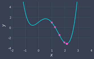
Here, we will run gradient descent for a total of 100 iterations. The result is as follows:

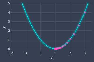
The final value of $x$ is $x^{(100)}\approx1$, which is what we would expect from visual inspection.

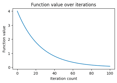
Plotting function value over iterations

The other way of visualizing how the function value changes over the iterations is to simply plot them:

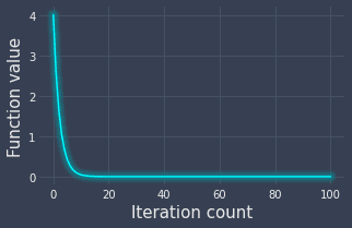
We can see that we nearly reach the minimum value at the 10th iteration!

Ideal value of learning rate

There is no one ideal value for $\alpha$ - while a specific alpha might work well for one situation, it may perform terribly for some other situation. For instance, if we set $\alpha=1$, then we end up in an infinite loop of going back and forth between $x=3$ and $x=-1$:

Therefore, it is important to test out different values of $\alpha$. Many machine learning libraries use a default learning rate of either $\alpha=0.01$ or $\alpha=0.001$.

NOTE

The gradient value becomes smaller as we approach the local minimum since the slope $f'(x)$ becomes flatter and approaches $0$. This means that we will take increasingly smaller steps as we iterate.

Gradient descent for two-dimensions

Suppose we wanted to minimize the following two-dimensional function:

$$f(x_0,x_1)=x_0^2+x_1^2$$

Visually, this looks like the following:

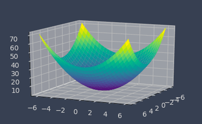
Visually, we can see that the minimum occurs at the origin $(0,0)$.

The principle equations for gradient descent would be as follows:

$$\begin{equation}\label{eq:bCLwwPiCj5oNFjNht6T} \begin{aligned} x_0^{(i+1)}&=x_0^{(i)}-\alpha\frac{\partial{f}}{\partial{x_0}}\\ x_1^{(i+1)}&=x_1^{(i)}-\alpha\frac{\partial{f}}{\partial{x_1}} \end{aligned} \end{equation}$$

Here, since we are dealing with multiple variables, we must switch to partial derivatives.

Just like for the one-dimensional case, we need to compute the gradients. Using basic calculus again, we can compute the two partial derivatives of our function $f$ with respect to $x_0$ and $x_1$ individually. Let's start by computing the partial derivative with respect to $x_0$:

$$\begin{align*} \frac{\partial{f}}{\partial{x}_0}&= \frac{\partial}{\partial{x}_0} (x_0^2+x_1^2)\\ &=2x_0 \end{align*}$$

Next, let's compute partial derivative with respect to $x_1$:

$$\begin{align*} \frac{\partial{f}}{\partial{x}_1}&= \frac{\partial}{\partial{x}_1} (x_0^2+x_1^2)\\ &=2x_1 \end{align*}$$

Therefore, we can update equations \eqref{eq:bCLwwPiCj5oNFjNht6T} as:

$$\begin{equation}\label{eq:fiGz17bpovyE0DUfacO} \begin{aligned} x_0^{(i+1)}&=x_0^{(i)}-2\alpha{x}_0^{(i)}\\ x_1^{(i+1)}&=x_1^{(i)}-2\alpha{x}_1^{(i)} \end{aligned} \end{equation}$$

Now that we have our principle equations, we must select a:

starting point - let's say $(x_0^{(0)}, x_1^{(0)})=(3,3)$.
learning rate - let's say $\alpha=0.05$.

Plugging our starting point and learning rate into \eqref{eq:fiGz17bpovyE0DUfacO} yields:

$$\begin{align*} x_0^{(1)}&=x_0^{(0)}-2\alpha{x}_0^{(0)}\\ &=3-2(0.05)(3)\\ &=2.7\\ x_1^{(1)}&=x_1^{(0)}-2\alpha{x}_0^{(1)}\\ &=3-2(0.05)(3)\\ &=2.7\\ \end{align*}$$

So after the first iteration, we end up at the point $(2.7,2.7)$.

In the next iteration, we compute the next position by applying the update equations \eqref{eq:fiGz17bpovyE0DUfacO} on our new point $(x_0^{(1)}, x_1^{(1)})=(2.7,2.7)$:

$$\begin{align*} x_0^{(2)}&=x_0^{(1)}-2\alpha{x}_0^{(1)}\\ x_1^{(2)}&=x_1^{(1)}-2\alpha{x}_1^{(1)} \end{align*}$$

We keep repeating this computation over and over again until some terminating condition is met. Let's assume that the terminating condition is 50 iterations. The following contour graph shows the movement of our point:

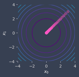
Here, the purplish contours in the middle represent lower values while the light-bluish outer contours represent higher values. As we can see, our point has gradually has moved towards the lowest point!

The final output of the gradient descent algorithm is the values of $x_0$ and $x_1$ that minimizes our function $f$:

$$\begin{align*} x^{(50)}_0&\approx0\\ x^{(50)}_1&\approx0 \end{align*}$$

Generalizing gradient descent for high dimensions

Up to now, we've covered gradient descent for one-dimensional and two-dimensional functions. Let's now generalize gradient descent to higher dimensions using vectors and matrices:

$$\begin{equation}\label{eq:mx0qJM7MMnbfHOzPLup} \boldsymbol{x}^{(i+1)}=\boldsymbol{x}^{(i)}-\alpha\nabla{f(\boldsymbol{x})} \end{equation}$$

Here $\nabla$ is the multi-variate version of the gradient. The expanded form of \eqref{eq:mx0qJM7MMnbfHOzPLup} is as follows:

$$\begin{pmatrix} x_0^{(i+1)}\\ x_1^{(i+1)}\\ \vdots\\ x_{n-1}^{(i+1)}\\ \end{pmatrix}= \begin{pmatrix} x_0^{(i)}\\ x_1^{(i)}\\ \vdots\\ x_{n-1}^{(i)}\\ \end{pmatrix}-\alpha \begin{pmatrix} \frac{\partial{f}}{\partial{x_0}}f(\boldsymbol{x})\\ \frac{\partial{f}}{\partial{x_1}}f(\boldsymbol{x})\\ \vdots\\ \frac{\partial{f}}{\partial{x_{n-1}}}f(\boldsymbol{x})\\ \end{pmatrix}$$

The logic behind gradient descent remains the same - we must compute the gradient $\nabla{f(\boldsymbol{x})}$, which holds the partial derivatives of $f$ with respect to each variable $x_0$, $x_1$ and $x_{n-1}$:

$$\frac{\partial{f}}{\partial{x_0}}f(\boldsymbol{x}), \frac{\partial{f}}{\partial{x_1}}f(\boldsymbol{x}),\cdots, \frac{\partial{f}}{\partial{x_{n-1}}}f(\boldsymbol{x})$$

Why gradient descent instead of gradient ascent?

As the name suggests, gradient descent is an optimization technique to find the minimum of a function. Gradient descent can also be used to find the maximum as well since we just need to flip the sign of the function. For instance, consider the problem of minimizing the function below:

$$\begin{equation}\label{eq:tPIr00yItjVlX2RZOi9} f(x)=(x-1)^2 \end{equation}$$

This optimization problem can be reformulated as maximizing the following function:

$$\begin{equation}\label{eq:Ir2dSfGPjkLPvPXvrFW} f(x)=-(x-1)^2 \end{equation}$$

The value that minimizes \eqref{eq:tPIr00yItjVlX2RZOi9} also maximizes \eqref{eq:Ir2dSfGPjkLPvPXvrFW}. In machine learning, we often deal with the cost function which we must minimize instead of maximizing Therefore, we usually use gradient descent instead of gradient ascent in machine learning.

Limitations of gradient descent

Getting stuck in a local minimum

A major limitation of gradient descent is that we can converge to a local minimum instead of a global minimum. For instance, consider the following function:

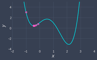
Here, we started at position $x=-1$ and we got stuck at a local minimum. If we had started at position $x=1$, we would reach the global minima instead:

The way to avoid getting stuck at a local minimum is to either:

re-run gradient descent using different starting points
use a more robust variant of gradient descent such as stochastic gradient descent. I will cover this variant soon - please join our newsletter by registering an accountopen_in_new!

Never converging

In some cases, the gradient descent will not converge. We have already come across this previously - this can happen when we go back and forth infinitely between two points:

Again, the way to overcome this limitation is to:

re-run gradient descent with different starting points
use another variant of gradient descent like stochastic gradient descent

Implementing gradient descent from scratch using Python's NumPy

Colab Notebook for Gradient Descent

Please log in or sign up to access the colab notebook

Click here to access all the code snippets in this section.

lock

The gradient descent implementation is surprisingly simple. Let's start with the one-dimensional case. Just as we did in our example above, suppose we wanted to perform gradient descent on the following function:

$$f(x)=(x-1)^2$$

We first begin by defining the function itself as well as its derivative:


        
        
            
                
                
                    def f(x):
  return (x-1) ** 2

def f_derivative(x):
  return (2*x)-2

We now implement the gradient descent algorithm:


        
        
            
                
                
                    import numpy as np

def gradient_descent(f, f_dash, init_x, alpha=0.01, step_num=100):
   x = init_x   # set the starting point of x
   res = [x]    # res will hold the x-value of each iteration
   for i in range(step_num):
       grad = f_dash(x)    # compute the gradient
       x -= alpha * grad   # update the value of x
       res.append(x)
   return x, np.array(res)

Note the following:

the five arguments are:
- f is the function we want to optimize ($f$)
- f_dash is the derivative function ($f'$)
- init_x is a number that represents the starting point ($x^{(0)}$)
- alpha is the learning rate ($\alpha$)
- step_num is the number of iterations to run
the two return values are:
- x is the final updated value of $x$
- np.array(res) is a NumPy array of the updated $x$-values from each iteration

We can use our gradient_descent(~) function like so:


        
        
            
                
                
                    x_min, hist_xs = gradient_descent(f, f_derivative, init_x=3)
print(f'Final x-value is {x_min}')
                
            
            Final x-value is 1.265239111789506

We can plot the function value against the iteration count by using the returned $x$-values of each iteration:


        
        
            
                
                
                    import matplotlib.pyplot as plt

ys = f(hist_xs)   # Compute the function values
plt.title('Function value over iterations')
plt.ylabel('Function value')
plt.xlabel('Iteration count')
plt.plot(np.arange(len(ys)), ys)   # The first argument is an array like [0,1,...,49]

This generates the following plot:

Computing the gradient numerically

In the previous implementation of gradient descent, we have explicitly defined the derivative function:


        
        
            
                
                
                    def f_derivative(x):
  return (2*x)-2

The problem with this approach is that the derivative function will obviously be different for other functions. Therefore, every time you want to run gradient descent on a function, you will have to manually work out the derivative function, which is tedious and error-prone.

What we can do instead is to numerically compute the approximate gradient like so:

$$f'(x)\approx\frac{f(x+h)-f(x-h)}{2h}$$

We can visualize how this works like so:

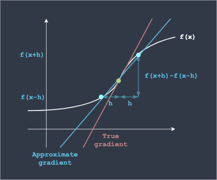
Here, $h$ is a small step taken to the left and right of the point to generate two points (colored blue in the diagram above) by which to compute the gradient. The calculation of the gradient is based on the classic approach of dividing the rise by the run.

The implementation of numerical differentiation in Python is dead simple:


        
        
            
                
                
                    def numerical_diff(f, x):
  h = 1e-4   # 0.0001
  return (f(x+h)-f(x-h))/(2*h)

NOTE

In theory, if we take $h$ to be infinitely small, the approximation of the gradient becomes exact. However, if we set the h to be too low in our code (e.g. h=1e-100), h will be rounded off to zero and throw a DivisionByZero error. This rounding-off happens because numerical types like float and double can only store a limited number of digits accurately.

Now, we can rewrite our gradient_descent(~) function to compute the gradient using numerical differentiation instead:


        
        
            
                
                
                    def gradient_descent(f, init_x, alpha=0.01, step_num=100):
   x = init_x
   res = [x]
   for i in range(step_num):
       grad = numerical_diff(f, x)
       x -= alpha * grad
       res.append(x)
   return x, np.array(res)

We can now conveniently just supply the function and the starting point:


        
        
            
                
                
                    x_min, xs = gradient_descent(f, 3)
print(f'Final x-value is {x_min}')
                
            
            Final x-value is 1.2652391117891397

Great, we see that the final value of $x$ is the same as before when we computed the gradient in exact form.

NOTE

There are two ways to perform differentiation - either numerically or analytically. Numerical differentiation involves computing the gradient approximately, whereas analytical differentiation involves computing the gradient by deriving an explicit derivative function. Analytical differentiation gives you the exact gradient value, while numerical differentiation returns only an approximate gradient value.

Generalizing to higher dimensions

The above gradient descent implementation is hard-coded to handle only the case of one dimension. We will now generalize our implementation to handle higher dimensions. To make things concrete, let's assume we are applying gradient descent on the following function:

$$f(x_0,x_1)=x_0^2+x_1^2$$

First and foremost, our target function will take as input a list of values instead of a single scalar:


        
        
            
                
                
                    def f(xs):
  return xs[0]**2 + xs[1]**2

Now, recall that the numerical differentiation for the one-dimensional case was as follows:

$$f'(x)=\frac{df}{dx}\approx\frac{f(x+h)-f(x-h)}{2h}$$

For the two-dimensional case, we will have to compute two partial derivatives, one with respect to the first dimension ($x_0$) and the other with respect to the second dimension ($x_1$):

$$\begin{align*} \frac{\partial{f}}{\partial{x_0}} =\frac{f(\begin{pmatrix} x_0+h\\ x_1\\ \end{pmatrix})-f(\begin{pmatrix} x_0-h\\ x_1\\ \end{pmatrix})}{2h}\\ \frac{\partial{f}}{\partial{x_1}} =\frac{f(\begin{pmatrix} x_0\\ x_1+h\\ \end{pmatrix})-f(\begin{pmatrix} x_0\\ x_1-h\\ \end{pmatrix})}{2h} \end{align*}$$

Here, note that we apply a small step $h$ on one specific dimension at a time (e.g. $x_0\pm{h}$ for the first partial derivative and $x_1\pm{h}$ for the second partial derivative). This logic extends to higher dimensional cases as well.

Next, we modify our implementation of numerical differentiation like so:


        
        
            
                
                
                    def f(xs):
  return xs[0]**2 + xs[1]**2

def numerical_diff(f, xs):
  h = 1e-4   # 0.0001
  grad = np.zeros_like(xs)
  for i in range(len(xs)):
    x = xs[i]
    xs[i] = x+h
    num_top = f(xs)   # Compute f(x+h)
    xs[i] = x-h
    num_bot = f(xs)   # Compute f(x-h)
    grad[i] = (num_top - num_bot) / (2*h)
    xs[i] = x   # Set the value back to the original
  return grad

Here, we are first creating a NumPy array grad that will hold our computed gradients using zeros_like(~). Since we are dealing with two-dimensional data, grad will be of length two and will initially be filled with zeros. We then iterate through each dimension using a simple for-loop. The core idea here is that we must make changes ($\pm{h}$) to one dimension at a time, and leave all the other dimensions intact. This involves setting the original value back for the current dimension at the end of each iteration.

We can use our new numerical_diff(~) function like so:


        
        
            
                
                
                    numerical_diff(f, [3,4])   # Returns a NumPy array
                
            
            array([6, 7])

Mathematically, we are computing the following:

$$\begin{align*} \frac{\partial{f}}{\partial{x_0}} =\frac{f(\begin{pmatrix} 3+0.005\\ 4\\ \end{pmatrix})-f(\begin{pmatrix} 3-0.005\\ 4\\ \end{pmatrix})}{2(0.005)}=6\\ \frac{\partial{f}}{\partial{x_1}} =\frac{f(\begin{pmatrix} 3\\ 4+0.005\\ \end{pmatrix})-f(\begin{pmatrix} 3\\ 4-0.005\\ \end{pmatrix})}{2(0.005)}=7 \end{align*}$$

Our function numerical_diff(~) returns a NumPy array containing these two partial derivatives.

Now, let's finally define our gradient descent function that uses this generalized version of numerical_diff(~):


        
        
            
                
                
                    def gradient_descent(f, init_xs, alpha=0.01, step_num=100):
   xs = init_xs
   res = [init_xs]
   for i in range(step_num):
      grad = numerical_diff(f, xs)
      xs -= alpha * grad
      res.append(xs)
   return xs, np.array(res)

From the outlook, nothing is different from the previous implementation of gradient_descent(~). However, the grad value returned by numerical_diff(~) was previously a numerical value, whereas now, grad value is a NumPy array holding the partial derivatives for each dimension.

We can use gradient_descent(~) like so:


        
        
            
                
                
                    best_xs, hist = gradient_descent(f, init_xs=[3,4], step_num=1000)
print(f'Final x-value is {best_xs}')
                
            
            Final x-value is [5.04890207e-09 6.74904257e-09]

The optimal value of $\boldsymbol{x}$ is approximately at the origin - we know this to be correct from our examplelink.

Closing thoughts

Gradient descent is an iterative algorithm that optimizes a given function. This technique plays an instrumental role in machine learning because many models define a cost function that we typically optimize via gradient descent.

In practice, other variants of the gradient descent algorithm (e.g. stochastic gradient descent) are used since the original version suffers from the limitationslink discussed above. If you want to be notified when I publish my weekly ML/DS comprehensive guide (e.g. about stochastic gradient descent), then please join our newsletter by registering an accountopen_in_new 🙂!

Published by Isshin Inada

Edited by 0 others

Did you find this page useful?

thumb_up

thumb_down

Comment

Citation

Ask a question or leave a feedback...

thumb_up

thumb_down

chat_bubble_outline

settings

Enjoy our search

Hit / to insta-search docs and recipes!