Suppose we toss an unfair coin three times. The probability that the coin lands on heads is $0.8$ . Compute the probabilities of tossing $0$ , $1$ , $2$ and $3$ heads.

Solution. Let's define the random variable $X$ as the number of heads obtained from the three tosses. The probabilities of tossing $0$ , $1$ , $2$ and $3$ heads are:

\begin{matrix} (1) & \begin{aligned} P (X = 0) & = P (TTT) \\ = 1 (0.8)^{0} (0.2)^{3} \\ P (X = 1) & = P (HTT or THT or TTH) \\ = P (HTT) \cdot P (THT) \cdot P (TTH) \\ = 3 (0.8)^{1} (0.2)^{2} \\ P (X = 2) & = P (HHT or HTH or THH) \\ = P (HHT) \cdot P (HTH) \cdot P (THH) \\ = 3 (0.8)^{2} (0.2)^{1} \\ P (X = 3) & = P (HHH) \\ = 1 (0.8)^{3} (0.2)^{0} \end{aligned} \end{matrix}

Let's understand how these probabilities were calculated. $P (X = 0)$ and $P (X = 3)$ are straight-froward because there is only one way to obtain $3$ tails or $3$ heads from $3$ tosses. Let's now focus on $P (X = 1)$ , which is the probability of obtaining $1$ heads. There are three ways to obtain $1$ heads:

HTT, THT, TTH

The key here is to realize that each of these outcomes occurs with the same probability.

\begin{aligned} P (HTT) & = (0.8)^{1} (0.2)^{2} \\ P (THT) & = (0.2)^{1} (0.8)^{1} (0.2)^{1} = (0.8)^{1} (0.2)^{2} \\ P (TTH) & = (0.2)^{2} (0.8)^{1} = (0.8)^{1} (0.2)^{2} \end{aligned}

Therefore, instead of computing all of these probabilities, we can simply compute one probability and multiply it by the number of ways to obtain the outcome. In this case, the number of ways of obtaining $1$ heads out of $3$ tosses is:

Number of ways of getting 1 head out of 3 trials = (\binom{3}{1}) = 3

If you are unfamiliar with the concept of combinations, please refer to our comprehensive guide here.

Similarly, for $P (X = 3)$ , we had to multiply the probabilities by the number of ways of getting $3$ heads out of $3$ tosses:

Number of ways of getting 3 heads out of 3 trials = (\binom{3}{3}) = 1

Let's now go back to and express the green multiples using combinations:

\begin{matrix} (2) & \begin{aligned} P (X = 0) & = (\binom{3}{0}) (0.8)^{0} (0.2)^{3} \\ P (X = 1) & = (\binom{3}{1}) (0.8)^{1} (0.2)^{2} \\ P (X = 2) & = (\binom{3}{2}) (0.8)^{2} (0.2)^{1} \\ P (X = 3) & = (\binom{3}{3}) (0.8)^{3} (0.2)^{0} \end{aligned} \end{matrix}

Can you see that there is a pattern here? In fact, we can compute each probability like so:

\begin{matrix} (3) & P (X = x) = (\binom{3}{x}) (0.8)^{x} (0.2)^{3 - x}, x = 0, 1, 2, 3 \end{matrix}

Here:

$3$ is the number of trials.
$0.8$ is the probability of success.
$0.2$ is the probability of failure.
$x$ is the number of successes we observe.

We can generalize $(3)$ by

replacing the number of trials ( $3$ ) with $n$ .
the probability of success ( $0.8$ ) with $p$ .
the probability of failure by ( $0.2$ ) with $1 - p$ .

Doing so will give us the famous binomial distribution below.

Definition.

Probability mass function of binomial distribution

A random variable $X$ is said to follow a binomial distribution if and only if the probability mass function of $X$ is:

p (x) = (\binom{n}{x}) p^{x} (1 - p)^{n - x}, x = 0, 1, 2, \dots, n

Where $n$ and $p$ are the parameters of the distribution defined as:

$n$ is the number of trials.
$p$ is the probability of success.

Note that we often use the notation $X \sim Bin (n, p)$ to denote that random variable $X$ follows a binomial distribution with parameters $n$ and $p$ .

Assumptions of binomial distribution

From our motivating example, it should be clear that the following conditions must be satisfied for the binomial distribution to be appropriate:

for each trial, there are only $2$ outcomes - either success or failure.
the number of trials $n$ is fixed.
each trial has the same probability of success $p$ . For instance, each time we toss a coin, the probability of getting a heads should always be the same.
each trial is independent, which means that the result of one trial does not affect the result of another. For instance, obtaining a heads in the current trial should not affect the probability of the outcome of the next coin trial.

Whenever these assumptions are satisfied, the experiment is called a binomial experiment. A single trial of a binomial experiment is called a Bernoulli trial. We will later look at Bernoulli random variables, which are special cases of the binomial random variables with number of trials $n = 1$ .

Example.

Rolling a dice

Suppose we roll a fair dice $3$ times. What is the probability of rolling a $4$ once?

Solution. Let's define the random variable $X$ as the number of $4$ s we roll. Let's check whether or not $X$ is binomially distributed:

each trial has either $2$ outcomes - either $4$ or not a $4$ . You may think that a dice roll has $6$ outcomes, but we are only concerned with the binary outcome of either $4$ or not $4$ .
the number of trials is fixed at $n = 3$ .
each trial has the same probability of success, $p = 1 / 6$ .
the trials are independent since the outcome of the current roll does not affect the outcome of the next roll.

Since the conditions of a binomial experiment are satisfied, $X$ is indeed a binomial random variable. Specifically, $X \sim Bin (3, 1 / 6)$ , which means that the probability mass function of $X$ is:

\begin{matrix} (4) & P (X = x) = (\binom{3}{x}) (\frac{1}{6})^{x} (\frac{5}{6})^{3 - x} \end{matrix}

The probability of rolling a $4$ once is therefore:

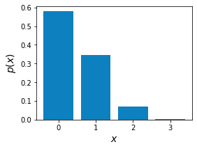
\begin{aligned} P (X = 1) & = (\binom{3}{1}) (\frac{1}{6})^{1} (\frac{5}{6})^{3 - 1} \\ = \frac{3!}{1! 2!} (\frac{1}{6}) (\frac{5}{6})^{2} \\ = 3 (\frac{1}{6}) (\frac{5}{6})^{2} \\ = \frac{25}{72} \\ \approx 0.35 \end{aligned}

We show the binomial probability mass function $(4)$ below:

We can see that the probability is indeed roughly $0.35$ for $x = 1$ . Intuitively, we should on average expect to roll a $4$ once every six rolls. Because we have only rolled $n = 3$ times, it makes sense that the probability that we don't roll a $4$ at all is the highest! Later on, we will dive deeper into what the expected value of a binomial random variable should be!

■

Example.

Case when binomial distribution does not apply

Suppose we have a bag that contains 3 red balls and 1 green ball. We randomly draw two balls in succession without replacement. If we let random variable $X$ denote the number of red balls we draw, does $X$ follow the binomial distribution?

Solution. Since we are not putting the ball back in for every trial, the probability of success (getting a red ball) changes. For instance, suppose we wanted to compute the probability of drawing two red balls. The probability of getting a red ball in the first draw is $3 / 4$ , and the probability of getting a red ball in the second draw is $2 / 3$ since we've taken the red ball out after the first draw. Therefore, the probability of drawing two red balls is:

P (X = 2) = (\frac{3}{4}) (\frac{2}{3})

This does not align with our formula for binomial distribution. In particular, this scenario violates the assumption of the binomial distribution that each trial is independent. Note that if the balls are drawn with replacement, that is, we put the ball back into the bag after each draw, then $X$ will follow a binomial distribution.

■

The Bernoulli distribution is a special case of the Binomial distribution where the number of trials $n$ is one. For instance, the outcome of a single coin toss can be represented by a Bernoulli random variable with a probability of heads $p$ .

Let's briefly discuss the properties of Bernoulli random variables as they will come in handy when deriving properties of Binomial random variables.

Theorem.

Bernoulli random variables

A random variable $X$ is said to be a Bernoulli random variable with parameter $p$ if and only if the probability mass function of $X$ is:

p (x) = {\begin{cases} 1 - p & for x = 0 \\ p & for x = 1 \end{cases}

Where $0 < p < 1$ . A Bernoulli random variable is denoted as $X \sim Ber (p)$ .

Intuition. The outcome of a Bernoulli random variable is either $0$ (failure) or $1$ (success). The outcome $0$ occurs with a probability of $1 - p$ and the outcome $1$ occurs with a probability of $p$ .

Here are two examples of Bernoulli random variables:

suppose we toss a fair coin once. If $X$ is a random variable such that $X = 1$ if heads (success) and $X = 0$ if tails (failure), then $X \sim Ber (1 / 2)$ .
suppose we roll a fair dice once. If $X$ is a random variable such that $X = 1$ if the outcome is one or two (success) and $X = 0$ otherwise (failure), then $X \sim Ber (2 / 6)$ .

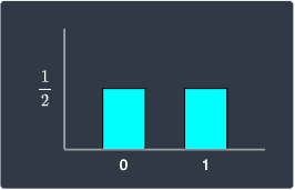
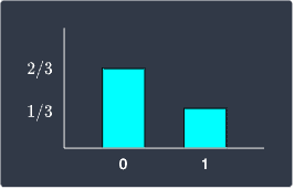
The probability mass function of the two examples are as follows:

$X \sim Ber (1 / 2)$	$X \sim Ber (1 / 3)$

Note that if we assume the bin widths to be one, the total area of the bins would add up to one!

■

Theorem.

Expected value and variance of Bernoulli random variables

If $X$ is a Bernoulli random variable with a probability of success $p$ , then the expected value and variance of $X$ are:

\begin{aligned} E (X) & = p \\ V (X) & = p (1 - p) \end{aligned}

Proof. Let's derive $E (X)$ first. Using the definition of expected values, we have that:

\begin{matrix} (5) & \begin{aligned} E (X) & = (1 - p) (0) + (p) (1) \\ = p \end{aligned} \end{matrix}

To derive variance $V (X)$ , let's use the following propertylink:

V (X) = E (X^{2}) - [E (X)]^{2}

We already know what $E (X)$ is, so let's derive $E (X^{2})$ . Using the definition of expected values once more, we have that:

\begin{aligned} E (X^{2}) & = (1 - p) 0^{2} + (p) 1^{2} \\ = p \end{aligned}

Substituting $E (X)$ and $E (X^{2})$ into $(5)$ gives us the variance:

\begin{aligned} V (X) & = p - p^{2} \\ = p (1 - p) \end{aligned}

This completes the proof.

■

Now, let's get back to exploring the properties of binomial random variables!

Theorem.

Expected value and variance of a binomial random variable

The expected value and variance of a binomial random variable $X \sim Bin (n, p)$ are:

\begin{aligned} E (X) & = n p \\ V (X) & = n p (1 - p) \end{aligned}

Proof. Perhaps the simplest and the most elegant way to derive the expected value and variance of a binomial random variable $X \sim Bin (n, p)$ is to treat them as the sum of $n$ independent Bernoulli random variables with a probability $p$ of success.

For instance, suppose we tossed a fair coin $3$ times. If we let random variable $X$ represent the total number of heads, then $X \sim Bin (3, 0.5)$ . However, the outcome of each toss can be represented by a Bernoulli random variable $Y_{i}$ where $Y_{i} = 1$ if heads and $Y_{i} = 0$ if tails - each of these outcomes occur at a probability of $0.5$ . Therefore, the binomial random variable $X$ can be expressed as the sum of three independent Bernoulli random variables:

X = Y_{1} + Y_{2} + Y_{3}

Let's go back to the general case when $X \sim Bin (n, p)$ . Again, $X$ can be expressed as the sum of $n$ independent Bernoulli random variables:

\begin{matrix} (6) & X = Y_{1} + Y_{2} + \dots + Y_{n} \end{matrix}

Taking the expected value of both sides and using the linearity of expected values:

\begin{matrix} (7) & \begin{aligned} E (X) & = E (Y_{1} + Y_{2} + \dots + Y_{n}) \\ = E (Y_{1}) + E (Y_{2}) + \dots + E (Y_{n}) \end{aligned} \end{matrix}

We have already provenlink earlier that the expected value of a Bernoulli random variable $Y_{i} \sim Ber (p)$ is:

\begin{matrix} (8) & E (Y_{i}) = p \end{matrix}

Plugging this into $(7)$ gives us the expected value of $X$ :

E (X) = n p

* * *

To derive the variance of our Binomial random variable $X$ , we can again use $(6)$ - but this time, we take the variance of both sides:

V (X) = V (Y_{1} + Y_{2} + \dots + Y_{n})

Because $Y_{1}, Y_{2}, \dots, Y_{n}$ are independent, we can use this propertylink of variance to get:

\begin{matrix} (9) & V (X) = V (Y_{1}) + V (Y_{2}) + \dots + V (Y_{n}) \end{matrix}

We have previously shownlink that the variance of a Bernoulli random variable $Y_{i} \sim Ber (p)$ is:

V (Y_{i}) = p (1 - p)

Plugging this into $(9)$ gives us the variance of $X$ :

V (X) = n p (1 - p)

This completes the proof.

■

Effects of parameters on the shape of the distribution

Increasing the sample size

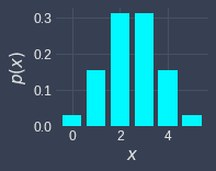
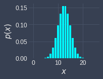
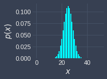
Increasing the sample size $n$ causes the probability mass function of a binomial random variable to take on a bell-curve shape:

$X \sim Bin (5, 0.5)$	$X \sim Bin (25, 0.5)$	$X \sim Bin (50, 0.5)$

Here, the probability of success is fixed at $p = 0.5$ , but the sample size is $n = 5, 25, 50$ from left to right, respectively. We can see that the probability mass function is starting to look like a continuous curve already at $n = 50$ . Although we won't do so here, we can mathematically prove that the binomial distribution converges to a normal distribution when the sample size $n$ is large.

Increasing probability of success

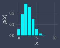
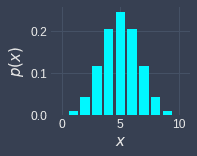
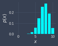
Increasing the probability of success $p$ causes the probability mass function of a binomial random variable to shift to the right:

$X \sim Bin (10, 0.25)$	$X \sim Bin (10, 0.50)$	$X \sim Bin (10, 0.75)$

Here, the sample size is fixed at $n = 10$ , but we vary the probability of success from $p = 0.25, 0.50, 0.75$ from left to right, respectively. This shifting behavior makes sense because the higher probability of success, the more successes we should expect.

Working with binomial random variables using Python

Computing the binomial probability mass function

Recall the following example question from earlier:

Suppose we roll a fair dice $3$ times. What is the probability of rolling a $4$ once?

We can define a binomial random variable $X \sim Bin (3, 1 / 6)$ to represent the number of times we roll a $4$ . The probability of rolling a $4$ once is therefore:

\begin{aligned} P (X = 1) & = (\binom{3}{1}) (\frac{1}{6})^{1} (\frac{5}{6})^{3 - 1} \\ \approx 0.35 \end{aligned}

We can also use a statistical library in Python called SciPy to easily compute the value of the binomial probability mass function:



            filter_none
            Copy

        
        
        
            
                
                
                    from scipy.stats import binom

n = 3
p = (1/6)
x = 1
binom.pmf(x, n, p)
                
            
            0.3472222222222223

Notice how this aligns with our hand-calculated result!

Drawing the binomial probability mass function

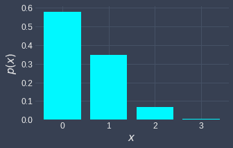
Consider the probability mass function of $X \sim Binom (3, 1 / 6)$ :

P (X = x) = (\binom{3}{x}) (\frac{1}{6})^{x} (\frac{5}{6})^{3 - x}

We can call the binom.pmf(~) function for all the possible values of $x$ like so:



            filter_none
            Copy

        
        
        
            
                
                
                    import matplotlib.pyplot as plt

n = 3
p = (1/6)
xs = list(range(n+1))   # [0,1,2,3]
# Calculate the pmf values and store in a list
pmfs = binom.pmf(xs, n, p)
# Plotting a bar chart with Matplotlib
plt.bar(xs, pmfs)
plt.xlabel('$x$')
plt.ylabel('$p(x)$')
plt.show()

This generates the following plot:

Published by Isshin Inada

Edited by 0 others

Did you find this page useful?

thumb_up

thumb_down

Comment

Citation

Ask a question or leave a feedback...

thumb_up

thumb_down

chat_bubble_outline

settings

Enjoy our search

Hit / to insta-search docs and recipes!