Now, suppose we play a game where we get $3$ dollars per heads and $4$ dollars per tails. Whether we get a heads or tails is random, so we can use random variable $X$ to denote the profit of a single toss. The probability mass function of $X$, denoted as $p(x)$, is as follows:

Outcome	$x$	$p(x)$
Heads	$3$	$0.8$
Tails	$4$	$0.2$

This table states that for a single toss:

the probability of getting $3$ dollars is $0.8$.
the probability of getting $4$ dollars is $0.2$.

Note that $x$ represents a specific value that a random variable $X$ could take on.

Now, the key question we wish to answer is:

If we toss the coin $n=10$ times, how much do we expect to profit?

To answer this question, we should first find out how many heads and tails we expect from $10$ tosses. Intuitively, since the probability of heads is $0.8$, we should expect the outcome to be $8$ heads and $2$ tails. Mathematically, we are performing the following calculations:

$$\begin{align*} \color{red}\text{Expected number of heads}&= n\times{p(3)}\\ &=(10)(0.8)\\ &=8\\\\ \color{green}\text{Expected number of tails} &=n\times{p(4)}\\ &=(10)(0.2)\\&=2\\ \end{align*}$$

Keep in mind that these are only the expected outcome since the outcome is random. Because we profit $3$ dollars for each heads and $4$ dollars for each tails, we can easily calculate the expected profit from heads and the expected profit from tails:

$$\begin{align*} \color{purple}\text{Expected profit from heads}&= ({\color{red}\text{Expected number of heads}})\times(\text{Profit per heads})\\ &=(8)(3)\\ &=24\\\\ \color{orange}\text{Expected profit from tails}&= ({\color{green}\text{Expected number of tails}})\times(\text{Profit per tails})\\ &=(2)(4)\\ &=8 \end{align*}$$

The sum of the expected profits from heads and tails gives us the total expected profit:

$$\begin{align*} \text{Expected profit} &= {\color{purple}\text{Expected profit from heads}}+ {\color{orange}\text{Expected profit from tails}}\\ &=24+8\\ &=32\\ \end{align*}$$

Therefore, if we were to toss the coin $10$ times, then our expected profit is $32$ dollars! We can generalize the above calculations as follows:

$$\begin{align*} \text{Expected profit} &=\overbrace{\underbrace{[n\times{p(3)}]}_{\text{Expected number of X=3}}\times{3}}^{\text{Expected profit of X=3}} +\overbrace{\underbrace{[n\times{p(4)}]}_{{\text{Expected number of X=4}}}\times{4}}^{\text{Expected profit of X=4}} \end{align*}$$

Now, instead of tossing the coin $n=10$ times, let's calculate the expected profit from a single coin toss, that is, $n=1$. Plugging in $n=1$ in the above formula gives:

$$\begin{equation}\label{eq:Btv5DtOEWn7AzPrgmka} \text{Expected profit of a single trial} =3\cdot{p(3)}+4\cdot{p(4)} \end{equation}$$

Recall that the random variable $X$ represents the profit of a single trial. We can mathematically denote the expected value of $X$ as $\mathbb{E}(X)$, which in this case means:

$$\begin{equation}\label{eq:rOdh5mI4gWAOeRva7TV} \mathbb{E}(X)= \text{Expected profit of a single trial} \end{equation}$$

Moreover, notice how the right-hand side of \eqref{eq:Btv5DtOEWn7AzPrgmka} can be written as:

$$\begin{equation}\label{eq:Ln9S8Mcey8PttjlMMnf} \sum_x{x\cdot{p(x)}} =3\cdot{p(3)}+4\cdot{p(4)} \end{equation}$$

Here, the summation symbol $\sum_x$ means that we are summing over all possible values of $x$.

Therefore, using \eqref{eq:rOdh5mI4gWAOeRva7TV} and \eqref{eq:Ln9S8Mcey8PttjlMMnf}, we can express \eqref{eq:Btv5DtOEWn7AzPrgmka} generally as:

$$\mathbb{E}(X) =\sum_x{x\cdot{p(x)}}$$

For our example, we know that $p(3)=0.8$ and $p(4)=0.2$, so the expected profit for a single toss is:

$$\begin{align*} \mathbb{E}(X) &=\sum_{x}x\cdot{p(x)}\\ &=(3)\cdot{p(3)}+(4)\cdot{p(4)}\\ &=(3)(0.8)+(4)(0.2)\\ &=3.2 \end{align*}$$

Therefore, we should expect to profit $3.2$ dollars per toss on average! Note that this does not mean that we get $3.2$ dollars per toss - in fact, that's impossible because we either get $3$ or $4$ dollars per toss. An expected profit of $3.2$ dollars per toss means that if we were to toss the coin a large number of times, the average profit we make per toss is $3.2$ dollars.

Simulation to demonstrate expected values

Let's run a quick simulation to demonstrate this. Suppose we toss the coin $1000$ times - the simulated outcome is as follows:

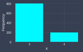
As expected, we get around $800$ heads ($X=3$) and $200$ tails ($X=4$). Below is a graph showing the running average of the profit per toss:

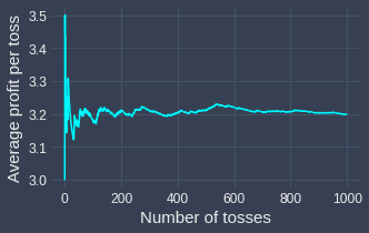
We can see that the average profit per toss fluctuates a lot in the beginning. However, as we keep tossing the coin, the average profit per toss stabilizes to the theoretical expected value of $3.2$ that we calculated earlier! The more tosses we make, the closer the average profit per toss will be to $3.2$.

In this example, the random variable $X$ represents the profit from a single toss and so $\mathbb{E}(X)$ represents the expected profit from a toss. Of course, $X$ does not have to represent profit - it could for instance represent waiting time, in which case $\mathbb{E}(X)$ would represent the expected waiting time.

We now state the formal definition of the expected value of random variables.

Definition.

Expected value of a random discrete variable

Let $X$ be a discrete random variable with probability mass function $p(x)$. The expected value of $X$ is defined as follows:

$$\mathbb{E}(X)=\sum_{x}{x\cdot{p(x)}}$$

In words, the expected value involves summing the products of all possible values of the random variable $X$ and their respective probability. Intuitively, the expected value of $X$ is a number that tells us the average value of $X$ we expect to see when we perform a large number of independent repetitions of an experiment.

Note that $\mathbb{E}(X)$ is sometimes denoted as $\mu$.

Example.

Expected profit from a lottery

Consider a lottery game where the cost of a single ticket is $3$ dollars. Let the random variable $X$ denote the lottery prize. The following table describes the three possible outcomes and their corresponding probabilities:

$x$	$p(x)$
$0$	$0.90$
$10$	$0.08$
$100$	$0.02$

Compute and interpret the expected value of $X$.

Solution. By definition, the expected value of $X$ is:

$$\begin{align*} \mathbb{E}(X) &=\sum_{x}x\cdot{p(x)}\\ &=(0)\cdot{p(0)}+(10)\cdot{p(10)}+(100)\cdot{p(100)}\\ &=(0)(0.9)+10(0.08)+100(0.02)\\ &= 2.8 \end{align*}$$

This means that we should expect to win $2.8$ dollars per lottery game. However, since the cost of a single lottery ticket is $3$ dollars, we will lose $0.2$ dollars per game on average. If we play $100$ games, then we should expect to lose a total of $20$ dollars.

■

Example.

Expected waiting time for food

The waiting time (in minutes) for food delivery is represented by the random variable $X$. The probability mass function of $X$ is:

$x$	$p(x)$
$10$	$0.2$
$20$	$0.3$
$30$	$0.5$

On average, how long do we have to wait to get our food?

Solution. Let random variable $X$ be the waiting time for the food to arrive. The expected value of $X$ is:

$$\begin{align*} \mathbb{E}(X) &=\sum_xx\cdot{p(x)}\\ &=(10)(0.2)+(20)(0.3)+(30)(0.5)\\ &=2+6+15\\ &=23\\ \end{align*}$$

Therefore, on average, we must wait 23 minutes for our food!

■

Example.

Expected value of a symmetric distribution

Suppose we have a probability mass function like so:

$x$	$4$	$5$	$6$
$p(x)$	$1/4$	$2/4$	$1/4$

This is visualized below:

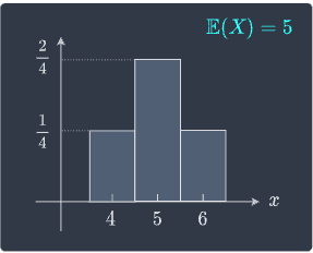
When we have symmetric distributions like this, we can find the expected value without having to calculate it. We know that the expected value is the mean value that a random variable takes in the long run. For a symmetric distribution, the mean is at the center, which means $\mathbb{E}(X)=5$.

Example.

Expected value of rolling a dice

Suppose we roll a fair dice once. Let the random variable $X$ denote the face of the rolled dice. What is the expected value of $X$?

Solution. Since we have a fair dice, the probability mass function of $X$ is:

$x$	$1$	$2$	$3$	$4$	$5$	$6$
$p(x)$	$1/6$	$1/6$	$1/6$	$1/6$	$1/6$	$1/6$

The expected value of $X$ is:

$$\begin{align*} \mathbb{E}(X) &=\sum_xx\cdot{p(x)}\\ &=(1)(1/6)+(2)(1/6)+(3)(1/6)+(4)(1/6)+(5)(1/6)+(6)(1/6)\\ &=3.5 \end{align*}$$

One way of interpreting this is to think of $X$ as points - for instance, if we roll a $6$, we get $6$ points. On average, we would get $3.5$ points per roll.

As a side note, notice that $p(x)$ is a symmetric probability distribution. We know from earlier that the expected value of a symmetric distribution is the mean value of $x$, that is:

$$\frac{1+2+3+4+5+6}{6}=3.5$$

This way of computing the expected value is convenient because we don't have to deal with probabilities - we simply compute the average of all possible $x$ values!

■

We will now discuss the expected values of continuous random variables. The underlying intuition is the same as that for the discrete case - the main difference is that instead of summing over all possible values of a random variable, we integrate over them!

Definition.

Expected value of a continuous random variable

Let $X$ be a continuous random variable with probability density function $f(x)$. The expected value of $X$ is defined as follows:

$$\mathbb{E}(X)=\int^\infty_{-\infty} x\cdot{f(x)}\;dx$$

Note the following:

this definition holds only if the integral exists.
the bounds of the integral are typically written as $-\infty$ and $\infty$ for the formal definition of expected values. In practice, we use the bounds of $X$ instead.

Example.

Computing the expected value of a continuous random variable (1)

Suppose random variable $X$ has the following probability density function:

$$f(x)= \begin{cases} \;2x,&0\le{x}\le1\\ \;0,&\text{elsewhere}\\ \end{cases}$$

Compute the expected value of $X$.

Solution. By definition, the expected value of $X$ is:

$$\begin{align*} \mathbb{E}(X) &=\int^\infty_{-\infty}x\cdot{f(x)}\;dx\\ &=\int^1_0x(2x)\;dx\\ &=2\int^1_0x^2\;dx\\ &=2\Big[\frac{x^3}{3}\Big]^1_0\\ &=2\Big(\frac{1}{3}\Big)\\ &=\frac{2}{3} \end{align*}$$

Therefore, if we repeatedly sample from this distribution a large number of times, the average value that $X$ will take on is $2/3$.

■

Example.

Computing the expected value of a continuous random variable (2)

Suppose random variable $X$ has the following probability density function:

$$f(x)= \begin{cases} 1/3,&5\le{x}\le8\\ 0,&\text{elsewhere} \end{cases}$$

Compute $\mathbb{E}(X)$.

Solution. By definition, the expected value of $X$ is:

$$\begin{align*} \mathbb{E}(X) &=\int^\infty_{-\infty}x\cdot{f(x)}\;dx\\ &=\int^8_5x\Big(\frac{1}{3}\Big)\;dx\\ &=\frac{1}{3}\int^8_5x\;dx\\ &=\frac{1}{3}\Big[\frac{x^2}{2}\Big]^8_5\\ &=\frac{1}{6}(64-25)\\ &=6.5 \end{align*}$$

Therefore, the average value that $X$ takes on in the long run is $6.5$.

Just as in the discrete case, we don't have to rely on the formula to compute the expected value when the distribution is symmetric. The probability density function of $X$ in this case is symmetric:

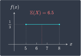
Because $\mathbb{E}(X)$ represents the average value that $X$ takes on upon repeated sampling, we have that $\mathbb{E}(X)$ must be at the center when the distribution of $X$ is symmetric. Therefore, we can easily conclude that $\mathbb{E}(X)=6.5$ in this case.

■

In the next section, we will go over the mathematical properties of expected value of random variables.

Published by Isshin Inada

Edited by 0 others

Did you find this page useful?

thumb_up

thumb_down

Comment

Citation

Ask a question or leave a feedback...

thumb_up

thumb_down

chat_bubble_outline

settings

Enjoy our search

Hit / to insta-search docs and recipes!