Cross validation is a technique to measure the performance of a model through resampling. It is a standard practice in machine learning to split the dataset into training and testing sets. The training set is used to train the model, while the testing set is used to evaluate the performance of the model. Cross validation extends this process by repeatedly splitting the dataset into different training and testing sets. Since cross validation ensures that all observations appear in the training and testing sets, the evaluation metric is considered to be more reliable.

The problem with a simple train-test split

To intuitively understand why cross validation is important, we must first understand why a simple train-test split can be problematic. Consider a classifier that predicts whether a review is negative, neutral or positive. Suppose that our dataset comprises of 40% negative reviews, 40% neutral reviews and 20% positive reviews. If we perform a train-test split with 80% training set and 20% testing set, the following scenario might happen:

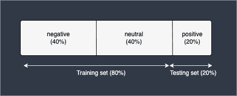
Here, the model will be trained using only negative and neutral reviews, and will be tested to see whether it can classify positive reviews correctly. Obviously, this split makes no sense because how can we expect a model to classify positive reviews when it has never seen any instances of them during training? Therefore, the testing accuracy in this case will be extremely low.

In fact, the opposite scenario can also happen. Suppose now that our dataset is comprised of 20% negative, 20% neutral and 60% positive reviews. With a simple 80-20 train-test split, we may end up with the following:

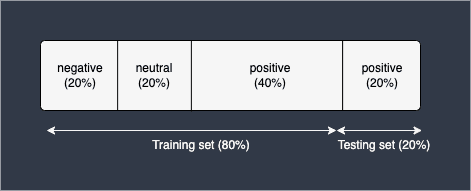
Here, the model has been trained on all three types of reviews, but unfortunately, the testing set comprises of positive reviews only. If the model happens to classify positive reviews extremely well, our testing accuracy will extremely high as well. This is, however, misleading because the model has only been tested on positive reviews thereby giving an inflated classification accuracy.

I admit that the two scenarios above are extreme, but who is to say such splits will never happen? In fact, there's a good chance that a more moderate version of these scenarios will happen in practise.

So how do we go about preventing these cases? The main cause is actually how the dataset was split - we randomly selected 80% of the data for training and the other 20% for testing. The problem with this is that the model's performance will be heavily influenced by this particular split, and so we cannot be certain that the model's performance will be similar if the split were to be different.

These situations can be prevented by cross validation, which uses different combinations of training and testing sets. With this approach, the model's performance can be measured using multiple splits instead of one particular split.

Algorithm of k-fold cross validation

The $k$-fold cross validation formalises this testing procedure. The steps are as follows:

Split our entire dataset equally into $k$ groups.
Use $k-1$ groups for the training set and leave one to use for the test set.
Train our model using our training set, and measure the performance using the training set.
Repeat steps 2 and 3 for a total of $k$ times, each time using a new group for the test set.
Compute the overall performance of our model by averaging the performance obtained in step 3.

Simple example of computing 4-fold cross validation

As an example, when $k=4$:

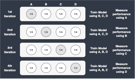
Here, note the following:

Suppose we had a dataset consisting of $100$ observations. Since $k=4$, $25$ observations will be used for testing, while $75$ observations will be used for training at each iteration.
The value of $k$ dictates the number of iterations, which means that the model must be trained $k$ number of times. This may be a problem for large datasets in which the training time is too long.
After $k$ iterations, we end up with $k$ number of performance metrics. Cross validation then simply computes the average of these to obtain a single performance metric.
Cross validation does not randomly split the dataset into training and testing sets - each observation will exactly appear once in the testing set in the entire process of cross validation.

A typical value set for $k$ is either $5$ or $10$. If the size of the dataset is small, then a larger value of $k$ is often set because more data can be used for training the model at each iteration.

Leave-one-out-cross-validation (LOOCV)

There exists a special case of the cross validation, called leave-one-out-cross-validation (LOOCV), in which the value of $k$ is set to $n$. For instance, suppose we have a dataset consisting of $100$ observations, and we perform LOOCV, that is, we set $k=100$. This means that at each iteration, $99$ observations will be used for training, while only $1$ observation will be used for testing. The total number of iterations in this case would be $100$.

LOOCV is often used when the size of the dataset is small since more observations can be used for training. Of course, the trade-off is that LOOCV is computationally expensive since the model must be trained a large number of times.

Performance Benchmarks

What we consider to be performance benchmarks would depend on our task at hand. Consider the following two cases:

regression problem
classification problem

Regression problem

Suppose we have a regression model (e.g. to predict a person's height). In this case, the mean squared error (MSE) is often used:

$$\mathrm{MSE}=\frac{1}{n}\sum_{i=1}^n(y_i-y ̂_i )^2$$

Where:

$n$ is the number of observations in the training set
$y_i$ is the actual label (e.g. a person's actual height)
$\hat{y}_i$ is the predicted value (e.g. a. person's predicted height by the model)

Classification problem

Suppose we have a classification model (e.g. to predict whether an e-mail is spam or not). In this case, we may want to use the misclassification error rate (MER):

$$\mathrm{MER}=\frac{1}{n}\sum^n_{i=1}I(\hat{y}_i\ne{y}_i)$$

Where:

$n$ is the number of observations in the training set
$I$ is what is known as the indicator function - more about this below
$y_i$ is the actual label (e.g. is the e-mail actually spam or not)
$\hat{y}_i$ is the predicted label

The indicator function allows us to express metrics like classification accuracy using mathematical equations:

$$I(\hat{y}_i\ne{y_i})=\begin{cases}1,& \hat{y}_i\ne{y}_i \\ 0, &\hat{y}_i={y}_i\end{cases}$$

In words, this indicator function does the following:

if the predicted label does not match with the actual label, the indicator function will evaluate to 1
if the predicted label matches with the actual label, the indicator function will evaluate to 0

Basically, the summation part in the equation for the $\text{MER}$ gives us the total number of misclassifications the model has made, and then dividing by $n$ will therefore give us the proportion of misclassified observations.

WARNING

As discussed in our article about confusion matrix, the performance metric to use largely depends on the scenario. For example, computing recall or precision instead may be more relevant.

Generalisation

We can take a general approach of defining a discrepancy function denoted as $D(\boldsymbol{y},\boldsymbol{\hat{y}})$, which measures the "distance" from $\boldsymbol{y}$ to $\boldsymbol{\hat{y}}$. The $\text{MSE}$ and $\text{MER}$ are just examples of this discrepancy function.

The cross validation error is defined like so:

$$\hat{\mathrm{Err}}_{\mathrm{cv}}=\frac{1}{k}\sum^k_{i=1}D(\boldsymbol{y}_i,\boldsymbol{\hat{y}}_i)$$

Remember, the $k$-fold cross validation will ultimately yield $k$ number of performance metrics since there will be $k$ iterations. Cross validation will then simply average these numbers to output a single performance metric.

Tuning hyper-parameters

Suppose we wanted to build a ridge regression model, which comes with one hyper-parameter - the penalty term ($\lambda$) - that requires tuning. We first come up with a list of values to use for the penalty terms - let's say:

$$\lambda=\{1,5,10,20\}$$

We then train our regression model based on each of these penalty terms using cross validation. For each of these models, we would end up with the corresponding validation error like so:

$\lambda$	Cross validation error
1	150
5	200
10	100
20	300

We can then compare the cross validation errors, and the optimal value of $\lambda$ would be the one with the lowest cross validation error. In this case, the optimal value would be $\lambda_{\text{opt}}=10$.

Comparing different models

Cross validation also allows us to compare any two models. For instance, suppose we have a classification problem, and we train two entirely different models – a neural network and a decision tree. Using cross validation, we can measure and compare the performance of both of these models. As a result, we can make an informed decision about which model is superior. This is in stark contrast to traditional statistical performance tests such as ANOVA, where we can only compare between nested models.

Cross validation using Python's sklearn

Basic example

Suppose we wanted to build a logistic regression classifier that predicts whether students will fail (0) or pass (1) an exam based on their GPA and number of hours studied. In order to evaluate the performance of our classifier, we will use 5-fold cross validation.

To begin, import the required libraries:


        
        
            
                
                
                    from sklearn.model_selection import KFold
from sklearn.model_selection import cross_val_score
from sklearn.linear_model import LogisticRegressionCV
import numpy as np
import pandas as pd

We then import the dataset from GitHub:


        
        
            
                
                
                    url = "https://raw.githubusercontent.com/SkyTowner/sample_data/main/binary_classification.csv"
df = pd.read_csv(url)
df.head()
                
            
                gpa   hours_studied  is_passed
0   2.2        9             0
1   2.4        3             0
2   3.1        2             0
3   3.2        9             0
4   3.1        6             0

We then split the DataFrame into features and the target:


        
        
            
                
                
                    X = df[["gpa","hours_studied"]]
y = df["is_passed"]

We then build our logistic regression model and perform cross validation:


        
        
            
                
                
                    # 5-fold cross validation
cv = KFold(n_splits=5, shuffle=True, random_state=42)
model_lr = LogisticRegressionCV(max_iter=1000)
scores = cross_val_score(model_lr, X, y, scoring='accuracy', cv=cv)
print(scores)
                
            
            [0.75  1.    0.875 0.75  0.875]

Here, note the following:

The shuffle=True means that X will initially be shuffled once before the resampling process happens. This is recommended because if the observations in the dataset are sorted by target, then each fold may contain observations from one class.
The cross_val_score(~) method returns a list of scores holding the classification accuracy (scoring='accuracy') of each iteration of the cross validation. Here, since $k=5$, and our dataset consists of 40 observations, each iteration uses 8 observations for testing, and 32 observations for training. There will be a total of 5 iterations, and this is the reason why the scores list contains 5 values.
Scikit-learn measures sets the classification threshold at 0.5 for binary classification. This means that if the model outputs 0.7 as a prediction for instance, then the predicted label would be 1. For multi-class classification, the class with the highest predicted probability will be chosen as the prediction label.

We can compute the mean classification accuracy by simply taking the average:


        
        
            
                
                
                    print('Accuracy: %.3f (%.3f)' % (np.mean(scores), np.std(scores)))
                
            
            Accuracy: 0.850 (0.094)

WARNING

Here, we have evaluated the classification accuracy by setting scoring='accuracy'. In order to specify multiple evaluation metrics, use cross_validate(~) introduced below.

Using cross_validate instead of cross_val_score

Instead of using cross_val_score(~) function, we could also use Sklearn's cross_validate(~) which returns more information than cross_val_score(~):


        
        
            
                
                
                    from sklearn.model_selection import cross_validate

result = cross_validate(model_lr, X, y, scoring='accuracy', cv=cv)
print(result)
                
            
            {
   'fit_time': array([0.30224562, 0.2726655 , 0.27249241, 0.27039385, 0.13665462]),
   'score_time': array([0.00281358, 0.00299811, 0.00291467, 0.00176215, 0.00163174]),
   'test_score': array([0.75 , 1.   , 0.875, 0.75 , 0.875])
}

Here:

fit_time is the time taken in seconds to fit and train the model
score_time is the time taken in seconds to evaluate the model using the testing set
test_score is the performance metric derived from the testing set. In this case, these numbers represent the classification accuracy as we have specified scoring='accuracy'. This is actually what cross_validate(~) returns.

Specifying multiple evaluation metrics

There are several ways to specify the multiple evaluation metrics.

Using a list

The easiest way to specify the evaluation metrics using a list of strings:


        
        
            
                
                
                    scores = cross_validate(model_lr, X, y, scoring=['accuracy', 'precision'], cv=cv)
print(scores)
                
            
            {
   'fit_time': array([0.16392016, 0.14529777, 0.14938974, 0.13513589, 0.1444366 ]),
   'score_time': array([0.00398898, 0.00389647, 0.00315475, 0.00281596, 0.00929856]),
   'test_accuracy': array([0.75 , 1.   , 0.875, 0.75 , 0.875]),
   'test_precision': array([0.6       , 1.        , 0.75      , 0.83333333, 1.        ])
}

Notice how the evaluation metrics are prefixed with test_.

Using a dictionary

We can also specify multiple evaluation metrics using a dictionary:


        
        
            
                
                
                    scoring = {
    'my_accuracy': 'accuracy',
    'prec': 'precision'
}

result = cross_validate(model_lr, X, y, scoring=scoring, cv=cv)
print(result)
                
            
            {
   'fit_time': array([0.40350699, 0.35918665, 0.29872012, 0.27520061, 0.55078173]),
   'score_time': array([0.00448251, 0.00518584, 0.0047617 , 0.00458765, 0.01307607]),
   'test_my_accuracy': array([0.75 , 1.   , 0.875, 0.75 , 0.875]),
   'test_prec': array([0.6       , 1.        , 0.75      , 0.83333333, 1.        ])
}

Notice how the key of our dictionary (e.g. 'prec') is attached to test_. The advantage of this approach is that you can specify the keys of the resulting scores.

Implementing a custom scoring function

To implement a custom scoring function, use Sklearn's make_scorer(~) function:


        
        
            
                
                
                    from sklearn.model_selection import cross_validate
from sklearn.metrics import make_scorer

def my_custom_score(y_true, y_predicted):
  ''' y_true is a Pandas Series
      y_predicted is a NumPy array '''
  num_misclassfications = np.sum(np.abs(y_true-y_predicted))
  num_predictions = len(y_true)
  return (num_misclassfications / num_predictions)

scorer = {
    'sklearn_accuracy': 'accuracy',
    'my_misclassification_error': make_scorer(my_custom_score, greater_is_better=False)
}

scores = cross_validate(model_lr, X, y, scoring=scorer, cv=cv)
print(scores)
                
            
            {
   'fit_time': array([0.31392479, 0.28502989, 0.29374075, 0.28535032, 0.29391599]),
   'score_time': array([0.00409293, 0.00416851, 0.00463891, 0.00447869, 0.00267291]),
   'test_sklearn_accuracy': array([0.75 , 1.   , 0.875, 0.75 , 0.875]),
   'test_my_misclassification_error': array([-0.25 , -0.   , -0.125, -0.25 , -0.125])
}

Here:

my_custom_score is a function that computes the misclassification error, which is simply one minus the classification accuracy.
Since a smaller misclassification error is better, we set greater_is_better=False.

Using cross_val_predict

We have so far looked at the usage of cross_validate and cross_val_score. We now look at cross_val_predict(~) that returns the predicted label of each sample:


        
        
            
                
                
                    from sklearn.model_selection import cross_val_predict

scores = cross_val_predict(model_lr, X, y, cv=cv)
print(scores)
                
            
            [0 0 0 1 0 0 0 0 0 0 0 0 0 0 0 1 0 1 0 1 1 0 1 1 1 1 1 1 1 1 1 1 1 1 1 1 1
 1 0 1]

Here, we have 40 samples in the dataset, and therefore we have 40 predicted labels. Remember, every sample occurs exactly once in the testing set, and so we will make exactly one prediction per sample.

Published by Isshin Inada

Edited by 0 others

Did you find this page useful?

thumb_up

thumb_down

Comment

Citation

Ask a question or leave a feedback...

thumb_up

thumb_down

chat_bubble_outline

settings

Enjoy our search

Hit / to insta-search docs and recipes!