Recall that the geometric distribution is the distribution of the number of trials to observe the first success in repeated independent Bernoulli trials. The negative binomial distribution generalizes this, that is, the negative binomial distribution is the distribution of the number of trials to observe the first $r$ successes in repeated independent Bernoulli trials.

Now, let's go over a simple example that will allow us to derive the probability mass function of the negative binomial distribution. Suppose have an unfair coin with the following probability of heads and tails:

$$\begin{align*} \mathbb{P}(\mathrm{H})&=0.2\\ \mathbb{P}(\mathrm{T})&=0.8\\ \end{align*}$$

Let's denote the outcome of heads as a success and the outcome of tails as a failure. Suppose we are interested in observing the $3$rd success at the $7$th trial. For this to be true, we must have observed $3-1=2$ successes in $7-1=6$ trials.

What is the probability of observing $2$ successes in $6$ trials? This should remind you of the binomial distribution, which applies in this case because:

the number of trials ($n=6$) is fixed.
the probability of success ($p=0.2$) is fixed.
the trials are independent.

The probability of observing $3-1$ successes in $7-1$ trials can therefore be computed using the binomial distribution:

$$\begin{equation}\label{eq:BN8wE2lZiSbMTrZic1d} \mathbb{P}(\text{Observing } 3-1 \text{ successes in }7-1\text{ trials})= \binom{7-1}{3-1}(0.2)^{7-1}(0.8)^{(7-1)-(3-1)} \end{equation}$$

Note that the reason why we don't compute $3-1$ and $7-1$ is so that we can generalize the formula later!

We also need to observe the $3$rd success at the $7$th trial, which means that the $7$th toss must result in a heads. The probability of this occurring is $p=0.2$, so we multiply \eqref{eq:BN8wE2lZiSbMTrZic1d} by $p=0.2$ to get:

$$\begin{equation}\label{eq:GSyRIKiU9e2CggQjrvt} \mathbb{P}(\text{Observing 3rd success at the 7th trial})= \binom{7-1}{3-1}(0.2)^{7-1}(0.8)^{(7-1)-(3-1)}\cdot{(0.2)} \end{equation}$$

Let's now generalize this. Suppose we perform repeated Bernoulli trials where the probability of success is $p$. The probability that the $r$-th success occurs on the $x$-th trial is given by:

$$\begin{align*} \mathbb{P}(\text{Observing }r\text{-th success at the }x\text{-th trial})&= \binom{x-1}{r-1}p^{r-1}(1-p)^{(x-1)-(r-1)}\cdot{p}\\ &= \binom{x-1}{r-1}p^{r}(1-p)^{(x-r)} \end{align*}$$

We assume that $r$ is given, and we denote the outcome of $x$ using a random variable $X$ like so:

$$\begin{equation}\label{eq:Ege1d4nAG8KS5d1nFLG} \mathbb{P}(X=x)= \binom{x-1}{r-1}p^{r}(1-p)^{(x-r)} \end{equation}$$

The minimum value that $x$ can take is $r$. For instance, the $r=3$ successes will take at least $x=3$ trials. Therefore, we have that $x=r,r+1,r+2,\cdots$. What we have managed to derive is the probability mass function of the negative binomial distribution!

Definition.

Negative Binomial Distribution

A random variable $X$ is said to follow a negative binomial distribution with parameters $(r,p)$ if and only if the probability mass function of $X$ is:

$$\mathbb{P}(X=x)= \binom{x-1}{r-1}p^{r}(1-p)^{(x-r)}, \;\;\;\;\;\;\; \text{for }\;x=r,r+1,r+2,\cdots$$

Where $0\le{p}\le1$.

Example.

Rolling a dice

Suppose we keep rolling a fair dice until we observe $3$ sixes in total. What is the probability that we roll a six for the $3$rd time at the $8$th roll?

Solution. Let's treat the event of observing a $6$ as a success. Since we have a fair dice, the probability of success is $1/6$. Let random variable $X$ represent the number of trials to observe the $3$rd success. Since rolling the fair dice is a binomial experiment, random variable $X$ follows the negative binomial distribution with parameters $r=3$ and $p=1/6$. Therefore, the probability mass function of $X$ is:

$$\begin{equation}\label{eq:kY8v1hT0ly6UJKz3Yic} \mathbb{P}(X=x) =\binom{x-1}{3-1}\Big(\frac{1}{6}\Big)^{3}\Big(1-\frac{1}{6}\Big)^{(x-3)}\\ \end{equation}$$

The probability of observing the $3$rd success at the $x=8^{\text{th}}$ trial is:

$$\begin{equation}\label{eq:c3w7Z2AQEsHfuNlLG4Y} \begin{aligned}[b] \mathbb{P}(X=8) &=\binom{8-1}{3-1}\Big(\frac{1}{6}\Big)^{3}\Big(1-\frac{1}{6}\Big)^{(8-3)}\\ &=\binom{7}{2}\Big(\frac{1}{6}\Big)^{3}\Big(\frac{5}{6}\Big)^5\\ &\approx0.04 \end{aligned} \end{equation}$$

Therefore, the probability of rolling the $3$rd six in the $8$th toss is around $0.04$. Such a low probability is expected because intuitively, it should take us $18$ rolls to observe $3$ sixes on average. We will later mathematically justify this intuition when we look at the expected value of negative binomial random variables.

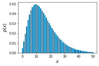
Let's also plot the negative binomial probability mass function \eqref{eq:kY8v1hT0ly6UJKz3Yic} below:

We can indeed see that when $X=8$, the probability is around $0.04$. I've truncated the plot at $X=50$, but there is no upper bound of $X$.

■

Properties of negative binomial distribution

Theorem.

Geometric distribution is a limiting case of the negative binomial distribution

If $X$ is a negative random variable with parameters $r=1$ and $p$, then $X$ is also a geometric random variable.

Proof. If $X$ is a negative random variable with parameters $r=1$ and $p$, then $X$ has the following probability mass function:

$$\begin{align*} \mathbb{P}(X=x) &=\binom{x-1}{r-1}p^{r}(1-p)^{x-r}\\ &=\binom{x-1}{1-1}p^{1}(1-p)^{x-1}\\ &=\binom{x-1}{0}p(1-p)^{x-1}\\ &=\frac{(x-1)!}{0!(x-1)!}p(1-p)^{x-1}\\ &=p(1-p)^{x-1}\\ \end{align*}$$

Notice that this is the probability mass function of the geometric distribution. Therefore, $X$ must be a geometric random variable. This completes the proof.

■

Theorem.

Mean of negative binomial distribution

If $X$ is a negative binomial random variable with parameters $(r,p)$, then the mean or expected value of $X$ is:

$$\mathbb{E}(X)=\frac{r}{p}$$

Proof. Most proofs for the mean and variance involve tedious algebraic manipulations, but we can avoid doing so by recognizing that the negative binomial distribution is the sum of independent geometric distributions. Let's take a moment to understand why.

Recall that the difference between the negative binomial distribution and geometric distribution is:

a negative binomial random variable $X$ represents the number of trials needed to observe $r$ successes.
a geometric random variable $Y$ represents the number of trials needed to observe the first success.

The diagram below illustrates the relationship between the two types of random variables:

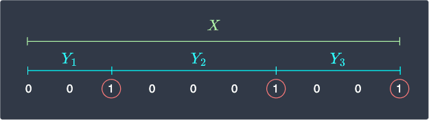
Here, a $0$ represents failure while a $1$ represents success. We can see that a negative binomial random variable with parameter $r$ can be decomposed as the sum of $r$ geometric random variables $Y_i$, that is:

$$\begin{equation}\label{eq:AVVJjcgLA9rjgDZXWXn} X=\sum^r_{i=1}Y_i \end{equation}$$

Note that the diagram above illustrates the case for $r=3$. Let's take the expected value of both sides of \eqref{eq:AVVJjcgLA9rjgDZXWXn} to get:

$$\begin{equation}\label{eq:cRVRXDUMtNyRzlN6jzN} \begin{aligned}[b] \mathbb{E}(X) &=\mathbb{E}\Big(\sum^r_{i=1}Y_i\Big)\\ &=\sum^r_{i=1}\mathbb{E}(Y_i) \end{aligned} \end{equation}$$

In our guide on geometric distribution, we have already provenlink that the expected value of a geometric random variable $Y_i$ is:

$$\begin{equation}\label{eq:MjOrhGKN5KVmQIqlAjW} \mathrm{E}(Y_i)=\frac{1}{p} \end{equation}$$

Where $p$ is the probability of success. Substituting \eqref{eq:MjOrhGKN5KVmQIqlAjW} into \eqref{eq:cRVRXDUMtNyRzlN6jzN} gives:

$$\begin{align*} \mathbb{E}(X) &=\sum^r_{i=1}\frac{1}{p}\\ &=\frac{r}{p}\\ \end{align*}$$

This completes the proof.

■

Theorem.

Variance of negative binomial distribution

If $X$ is a negative binomial random variable with parameters $(r,p)$, then the variance of $X$ is:

$$\mathbb{V}(X)=\frac{r(1-p)}{p^2}$$

Proof. We will again treat a negative random variable $X$ as a sum of the $r$ independent geometric random variables:

$$\begin{equation}\label{eq:mOy1plJPPNJYehXC97N} X=\sum^r_{i=1}Y_i \end{equation}$$

Let's take the variance of both sides:

$$\begin{equation}\label{eq:tk6ak4MTbRND65mClxz} \begin{aligned}[b] \mathbb{V}(X) &=\mathbb{V}\Big(\sum^r_{i=1}Y_i\Big)\\ &=\mathbb{V}(Y_1+Y_2+\cdots+Y_r)\\ &=\mathbb{V}(Y_1)+\mathbb{V}(Y_2)+\cdots+\mathbb{V}(Y_r)\\ &=\sum^r_{i=1}\mathbb{V}(Y_i) \end{aligned} \end{equation}$$

Note that the third equality holds by propertylink of variance because the geometric random variables are independent.

In our guide on geometric distribution, we have already provenlink that the variance of a geometric random variable $Y_i$ is:

$$\begin{equation}\label{eq:V3zEGxF346HAN9EYq44} \mathbb{V}(Y_i)=\frac{1-p}{p^2} \end{equation}$$

Finally, substituting \eqref{eq:V3zEGxF346HAN9EYq44} into \eqref{eq:tk6ak4MTbRND65mClxz} gives:

$$\begin{align*} \mathbb{V}(X) &=\sum^r_{i=1}\frac{1-p}{p^2}\\ &=\frac{r(1-p)}{p^2} \end{align*}$$

This completes the proof.

■

Example.

Rolling a dice (revisited)

Let's revisit our examplelink from earlier - suppose we keep rolling a fair dice until we roll a six for the $3$rd time. If we let random variable $X$ represent the number of trials to observe $r=3$ successes, then $X$ follows a negative binomial distribution with parameters $r=3$ and $p=1/6$.

We computed the probability of rolling a six for the $3$rd time at the $x=8^\text{th}$ roll to be:

$$\mathbb{P}(X=8)\approx0.04$$

We said that such a low probability is to be expected because it should, on average, take us $18$ rolls to observe $3$ sixes. This intuition of ours can now be justified mathematically by computing the expected value of $X$, that is:

$$\begin{align*} \mathbb{E}(X) &=\frac{r}{p}\\ &=\frac{3}{1/6}\\ &=18 \end{align*}$$

No wonder it's extremely rare to observe the $3$rd six at the $8$th roll!

Theorem.

Alternate parametrization of the negative binomial distribution

A random variable $X$ is also said to follow a negative binomial distribution with parameters $(r,p)$ if the probability mass function of $X$ is:

$$\mathbb{P}(X=x)= \binom{x+r-1}{r-1} p^r(1-p)^x, \;\;\;\;\;\;\; \text{for }\;x=0,1,2,\cdots$$

Where $0\le{p}\le1$.

Proof and intuition. The negative binomial distribution is sometimes formulated in a different way - instead of counting the number of trials at which the $r$-th success occurs, we can also count the number of failures before the $r$-th success.

For instance, observing the $3$rd success at the $5$th trial is logically equivalent to observing $5-3=2$ failures before observing the $3$rd success. This is illustrated below:

Let's now go the other way - observing $2$ failures before observing the $3$rd success is the same as observing the $3$rd success in the $(2+3)^{\text{th}}$ trial.

To generalize, let random variable $X$ represent the number of failures before observing the $r$-th success. This means that the $r$-th success occurs at the $(X+r)^{\text{th}}$ trial. We already know that $X+r$ follows a negative binomial distribution:

$$\begin{equation}\label{eq:UG3DpIrcX1s5jvmGzEK} \mathbb{P}(X+r=x+r)= \binom{(x+r)-1}{r-1}p^{r}(1-p)^{((x+r)-r)} \end{equation}$$

Let's simplify this, starting with the left-hand side:

$$\mathbb{P}(X+r=x+r)=\mathbb{P}(X=x)$$

We then simplify the right-hand side:

$$\binom{(x+r)-1}{r-1}p^{r}(1-p)^{((x+r)-r)}= \binom{x+r-1}{r-1}p^{r}(1-p)^{x}$$

Therefore, \eqref{eq:UG3DpIrcX1s5jvmGzEK} is:

$$\mathbb{P}(X=x)= \binom{x+r-1}{r-1} p^r(1-p)^x$$

Remember, $X$ represents the number of failures before observing the $r$-th success. This means that the values $X$ can take is $X=0,1,2,\cdots$. Note that this is quite different from the values $X$ can take for the first definition of the negative binomial distribution, which was $X=r,r+1,r+2,\cdots$.

■

Theorem.

Expected value and variance

The expected value and variance of the second definition of the negative binomial random variable are:

$$\begin{align*} \mathbb{E}(X)&=\frac{r(1-p)}{p}\\ \mathbb{V}(X)&=\frac{r(1-p)}{p^2} \end{align*}$$

Proof. We've already derived the expected value and variance of the first definition of the negative binomial random variable $X$. We know that $X-r$ follows the second definition of the geometric distribution, so all we need to do is to compute $\mathbb{E}(X-r)$ and $\mathbb{V}(X-r)$. We start with the expected value first:

$$\begin{align*} \mathbb{E}(X-r) &=\mathbb{E}(X)-r\\ &=\frac{r}{p}-r\\ &=\frac{r(1-p)}{p}\\ \end{align*}$$

The variance of $X-r$ is:

$$\begin{align*} \mathbb{V}(X-r) &=\mathbb{V}(X)\\ &=\frac{r(1-p)}{p^2} \end{align*}$$

The first equality holds by propertylink of variance because $r$ is some constant. This completes the proof.

■

Theorem.

Overdispersion

The variance of the second definition of a negative binomial random variable is always greater than its expected value, that is:

$$\mathbb{V}(X)\ge\mathbb{E}(X)$$

This is known as the overdispersion property of the negative binomial distribution.

Proof. We have derived the expected value and variance of the second definition of a negative binomial random variable to be:

$$\begin{align*} \mathbb{E}(X)&=\frac{r(1-p)}{p}\\ \mathbb{V}(X)&=\frac{r(1-p)}{p^2} \end{align*}$$

We can easily express the variance in terms of the expected value:

$$\mathbb{V}(X)=\frac{1}{p}\cdot\mathbb{E}(X)$$

Since $0\le{p}\le1$, we conclude that:

$$\mathbb{V}(X)\ge\mathbb{E}(X)$$

Note that the overdispersion property only applies to the case when we use the second definition of the geometric random variable.

■

Working with negative binomial distribution using Python

Computing the probability mass function

Recall the examplelink from earlier once more:

Suppose we keep rolling a fair dice until we observe $3$ sixes in total. What is the probability that we roll a six for the $3$rd time at the $8$th roll?

To align with Python's SciPy library, let's use the second parametrization of the negative binomial distribution to answer this question. We let random variable $X$ be the number of failures before observing the $r$-th success.

Observing the $3$rd success at the $8$th trial is equivalent to observing $8−3=5$ failures before observing the $3$rd success. Therefore, the probability of interest is given by:

$$\begin{align*} \mathbb{P}(X=5)&= \binom{5+3-1}{3-1} \Big(\frac{1}{6}\Big)^3\Big(1-\frac{1}{6}\Big)^5\\ &\approx0.039 \end{align*}$$

Instead of calculating by hand, we can use Python's SciPy library like so:


        
        
            
                
                
                    from scipy.stats import nbinom
r = 3
p = (1/6)
x = 5
nbinom.pmf(x,r,p)
                
            
            0.03907143061271146

Plotting the probability mass function

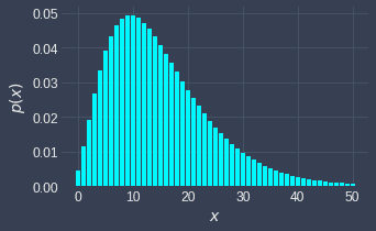
Suppose we wanted to plot the probability mass function of random variable $X$ that follows the second parametrization of the negative binomial distribution with $r=3$ and $p=1/6$ given below:

$$\mathbb{P}(X=x)= \binom{x+3-1}{3-1} \Big(\frac{1}{6}\Big)^3\Big(1-\frac{1}{6}\Big)^x, \;\;\;\;\;\;\; \text{for }\;x=0,1,2,\cdots$$

We can call the nbinom.pmf(~) function on a list of non-negative integers:


        
        
            
                
                
                    import matplotlib.pyplot as plt

r = 3
p = (1/6)
n = 50
xs = list(range(n+1))   # [0,1,2,...,50]
pmfs = nbinom.pmf(xs, r, p)
plt.bar(xs, pmfs)
plt.xlabel('$x$')
plt.ylabel('$p(x)$')
plt.show()

This generates the following plot:

Published by Isshin Inada

Edited by 0 others

Did you find this page useful?

thumb_up

thumb_down

Comment

Citation

Ask a question or leave a feedback...

thumb_up

thumb_down

chat_bubble_outline

settings

Enjoy our search

Hit / to insta-search docs and recipes!