

Comprehensive Guide on Variance of Random Variables
Start your free 7-days trial now!
To understand this guide, you must be familiar with the concept of expected values. Please consult our guide if you are not.
Variance of a random variable
If $X$ is a random variable with mean $\mathbb{E}(X)=\mu$, then the variance of a random variable $X$ is defined to be the expected value of $(X-\mu)^2$, that is:
Intuitively, we can think of the variance as the average squared distance between a random variable and its mean, measuring the spread of the random variable's distribution.
Intuition behind the variance formula
Recall that the expected value $\mathbb{E}(X)$ can be interpreted as the average value that $X$ takes when we repeatedly sample $X$ from its distribution. Therefore, $\mathbb{E}(X)$ is to be thought of as the mean of its distribution.
For example, suppose a random variable $X$ has the following probability mass function:
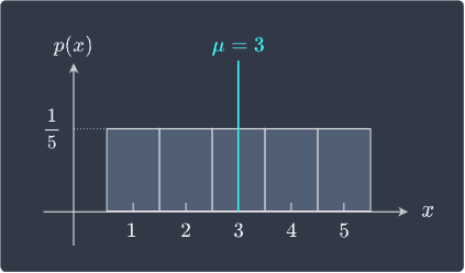
Recall from this sectionlink that the mean value $X$ for a symmetric probability distribution is at the center, which in this case is $\mathbb{E}(X)=\mu=3$.
Distance squared
The quantity $X-\mu$ measures the distance between a possible value of the random variable and the mean $\mu$. This is easy to calculate:
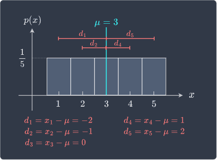
Notice how in the case when $X$ is smaller than the mean, the distance is negative. This is problematic for two reasons:
we only care about how far $X$ is from the mean $\mu$ and not the sign of the distance.
the positive and negative distances cancel out each other, which makes the average distance become zero, that is, $(1/5)\sum_{i=1}^5(x_i-\mu)=0$.
The second point implies that the expected value of $X-\mu$ is zero, which can also be shown using the linearity of expected values:
Clearly, this is not a good measure of spread because the probability histogram tells us that $x$ values are spread out, so the spread should not be equal to zero! Therefore, we should adjust the distance metric $X-\mu$ such that we don't encounter negative distances. One way of doing so is to take the square of $X-\mu$ like so:
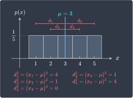
The quantity $(X-\mu)^2$ measures the squared distance between $X$ and the mean of $X$. Even though we have taken the square of the distance, $(X-\mu)^2$ is still a measure of how far $X$ is from the mean $\mu$.
Why take the square instead of the absolute value?
For those wondering why we don't take the absolute value of $X-\mu$ instead, it turns out that defining the variance as $(X-\mu)^2$ instead of $\vert{X-\mu}\vert$ leads to extremely useful properties such as:
None of these properties hold if we were to define the variance using absolute value.
Taking the expected value of the squared distance
We now know that $(X-\mu)^2$ is to be interpreted as the squared distance of $X$ from the mean of $X$ and is thus a measure of how far off $X$ is from the mean $\mu$. Taking the expected value of $(X-\mu)^2$ will therefore give us the average squared distance from the mean as we repeatedly sample $X$ from its distribution. This expected value is the definition of variance:
Let's now compute the variance of $X$. Recall the following propertylink of expected values:
If we define $g(X)=(X-\mu)^2$, then:
This allows us to compute the variance of $X$ like so:
Therefore, the measure of spread for $X$ is $2$. The higher this number, the more spread out $X$ is.
Comparing the spread of two random variables
Suppose we have two random variables $X$ and $Y$ and their distributions:
Low variance | High variance |
|---|---|
| 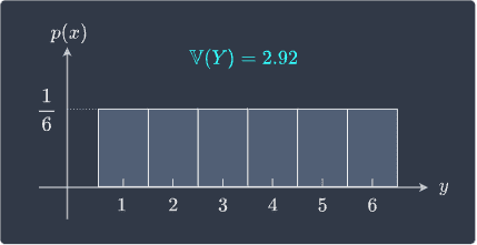
|
We can see that $Y$ is more spread out compared to $X$. Instead of having to rely on visual plots, we can mathematically show that $Y$ has more spread than $X$ since $\mathbb{V}(Y)\gt\mathbb{V}(X)$.
Rolling an unfair dice
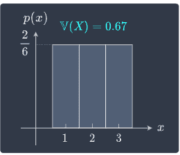
Suppose we rolled an unfair 3-sided dice with faces $1$, $2$ and $3$. Let random variable $X$ denote the outcome of the roll. We assume that $X$ has the following probability mass function:
$x$ | $p(x)$ |
|---|---|
$1$ | $1/6$ |
$2$ | $3/6$ |
$3$ | $2/6$ |
Compute the variance of $X$.
Solution. To compute the variance $\mathbb{V}(X)$ using its definition, we must first compute the mean of $X$, that is, $\mu$. By definitionlink of expected values, we have that:
Now, let's use the definition of variance:
Note that the definition of expected values is again used for the second equality.
Another measure of spread of a random variable is the standard deviation, which is defined as the square root of the variance. Variance is a more popular measure of spread because the variance has much nicer mathematical properties than standard deviation.
What's nice about standard deviation is that it has the same units as the random variable - for instance, if random variable $X$ has units of minutes, then the standard deviation would also be in minutes.
Standard deviation of a random variable
The standard deviation of a random variable $X$ is defined as the square root of the variance of $X$, that is:
Where $\mu$ is the mean or expected value of $X$.
In the next section, we will explore the mathematical properties of the variance of random variables!