Given a square matrix and a vector, we can easily verify whether or not the vector is an eigenvector of the matrix. Let's now go through some examples.

Example.

Verifying that a vector is not an eigenvector of a matrix

Suppose we have the following matrix and vector:

A = (\begin{matrix} 1 & 2 \\ 3 & 2 \end{matrix}), x = (\begin{matrix} 2 \\ 1 \end{matrix})

Show that $x$ is not an eigenvector of $A$ .

Solution. By definition, for $x$ to be an eigenvector of $A$ , the following equation must be satisfied:

A x = λ x

Where $λ$ is some scalar. Substituting our matrix and vector gives:

\begin{aligned} (\begin{array}{c} 1 & 2 \\ 3 & 2 \end{array}) (\begin{array}{c} 2 \\ 1 \end{array}) & = λ (\begin{array}{c} 2 \\ 1 \end{array}) \\ (\begin{array}{c} 4 \\ 8 \end{array}) & = λ (\begin{array}{c} 2 \\ 1 \end{array}) \end{aligned}

Clearly, the left vector is not a scalar multiple of the right vector, which means that a $λ$ satisfying the equation does not exist. Therefore, $x$ is not an eigenvector of $A$ .

■

Example.

Verifying that a vector is an eigenvector of a matrix

Suppose we have the following matrix and vector:

A = (\begin{matrix} 1 & 3 \\ 4 & 2 \end{matrix}), x = (\begin{matrix} 3 \\ 4 \end{matrix})

Show that $x$ is an eigenvector of $A$ .

Solution. Again, we check whether $A x = λ x$ holds for some scalar $λ$ like so:

\begin{aligned} (\begin{array}{c} 1 & 3 \\ 4 & 2 \end{array}) (\begin{array}{c} 3 \\ 4 \end{array}) & = λ (\begin{array}{c} 3 \\ 4 \end{array}) \\ (\begin{array}{c} 15 \\ 20 \end{array}) & = λ (\begin{array}{c} 3 \\ 4 \end{array}) \end{aligned}

We see that if $λ = 5$ , then the equation holds. Therefore, $x$ is an eigenvector of $A$ and the corresponding eigenvalue is $λ = 5$ .

Interestingly, $A$ may have other eigenvectors and eigenvalues as well. For instance, consider the same matrix $A$ but a different vector:

A = (\begin{matrix} 1 & 3 \\ 4 & 2 \end{matrix}), x^{'} = (\begin{matrix} - 1 \\ 1 \end{matrix})

Let's check whether $x^{'}$ is an eigenvector of $A$ or not:

\begin{aligned} (\begin{array}{c} 1 & 3 \\ 4 & 2 \end{array}) (\begin{array}{c} - 1 \\ 1 \end{array}) & = λ (\begin{array}{c} - 1 \\ 1 \end{array}) \\ (\begin{array}{c} 2 \\ - 2 \end{array}) & = λ (\begin{array}{c} - 1 \\ 1 \end{array}) \end{aligned}

This equation holds if $λ = - 2$ . Therefore, $x^{'}$ is indeed also an eigenvector of $A$ . We will later prove that an $n \times n$ matrix can have at most $n$ eigenvalues and corresponding eigenvectors.

■

As we have just demonstrated, verifying whether or not the given vector is an eigenvector of a matrix is easy. We will later introduce a procedure by which we can derive the eigenvalues and eigenvectors of a given matrix, but let's first go through their geometric intuition.

Geometric intuition behind eigenvalues and eigenvectors

Recall from this sectionlink that multiplying vectors by a scalar $λ$ geometrically means that we either shrink or stretch the vector by a factor of $λ$ . This is illustrated below:

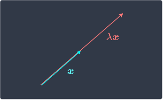
The matrix-vector product $A x$ can be thought of as a transformation by which $A$ converts $x$ into some other vector. In most cases, $A x$ results in a vector that has a different direction to $x$ , but eigenvectors are a special type of vectors that do not change direction but instead shrinks or stretches after the transformation.

We will now derive a method to compute the eigenvalues and eigenvectors of given a matrix.

Theorem.

Characteristic equation and polynomial

The characteristic equation of a square matrix $A$ is defined as:

\begin{matrix} (1) & det (A - λ I) = 0 \end{matrix}

Where:

$λ$ is an eigenvalue of $A$ .
$I$ is an identity matrix.

The left-hand side of $(1)$ is called the characteristic polynomial of $A$ - often denoted as $p_{A} (λ)$ .

Proof. By definition, for a given square matrix $A$ , its eigenvectors $x$ and eigenvalues $λ$ satisfy the following equation:

\begin{matrix} (2) & A x = λ x \end{matrix}

Remember, eigenvectors are defined to be non-zero, that is, not all elements in the vector are zero.

Let's rearrange $(2)$ to derive a formula that allows us to compute the eigenvalues:

\begin{matrix} (3) & \begin{aligned} A x & = λ x \\ A x - λ x & = 0 \\ A x - λ I x & = 0 \\ (A - λ I) x & = 0 \end{aligned} \end{matrix}

We are now going to assume that the matrix $A - λ I$ is invertible and thus has an inverse $(A - λ I)^{- 1}$ . Multiplying this inverse on both sides gives:

\begin{aligned} (A - λ I)^{- 1} (A - λ I) x & = 0 \\ I x & = 0 \\ x & = 0 \end{aligned}

This means that the eigenvector $x$ equals the zero vector. However, we started out by specifying that the eigenvector must be non-zero. Therefore, our assumption that $A - I λ$ is invertible is false. Since $A - I λ$ is not invertible, we know from theoremlink that the determinant of $A - λ I$ is zero:

\begin{matrix} (4) & \det (A - λ I) = 0 \end{matrix}

This equation is called the characteristic equation of $A$ . This completes the proof.

■

Computing eigenvalues

Observe how there is only one unknown value in $(4)$ - the eigenvalue $λ$ . Therefore, this is the equation that allows us to find the eigenvalues of a given matrix! Let's now go through an example.

Example.

Computing the eigenvalues of a 2x2 matrix

Compute the eigenvalues of the following matrix:

A = (\begin{matrix} 2 & 3 \\ 4 & 1 \end{matrix})

Solution. The characteristic equation of $A$ is:

\begin{aligned} det (A - λ I) & = 0 \\ det [(\begin{array}{c} 2 & 3 \\ 4 & 1 \end{array}) - λ (\begin{array}{c} 1 & 0 \\ 0 & 1 \end{array})] & = 0 \\ det [(\begin{array}{c} 2 - λ & 3 \\ 4 & 1 - λ \end{array})] & = 0 \end{aligned}

By theoremlink, we can compute the determinant of the $2 \times 2$ matrix:

\begin{aligned} (2 - λ) (1 - λ) - (3) (4) & = 0 \\ 2 - 2 λ - λ + λ^{2} - 12 & = 0 \\ λ^{2} - 3 λ - 10 & = 0 \\ (λ - 5) (λ + 2) & = 0 \\ λ & = 5, - 2 \end{aligned}

This means that the eigenvalues of $A$ are $5$ and $- 2$ . Typically, we label the eigenvalues using a subscript like so:

\begin{aligned} λ_{1} & = 5 \\ λ_{2} & = - 2 \end{aligned}

■

Computing eigenvectors

Now that we have found the eigenvalues of a given matrix $A$ , we must find the corresponding eigenvectors. Recall from $(3)$ that:

\begin{matrix} (5) & (A - λ I) x = 0 \end{matrix}

Here, $x$ is the eigenvectors that we are trying to find. Remember, $(5)$ holds for eigenvalues $λ_{1}$ and $λ_{2}$ . Let's substitute $λ = λ_{1}$ to get:

\begin{matrix} (6) & (A - λ_{1} I) x_{1} = 0 \end{matrix}

Here, we've added a subscript to $x_{1}$ to indicate that it is an eigenvector corresponding to the eigenvalue $λ_{1}$ . If $A$ is an $2 \times 2$ matrix, then the matrix form of $(6)$ is:

\begin{matrix} (7) & \begin{aligned} [(\begin{array}{c} a_{11} & a_{12} \\ a_{21} & a_{22} \end{array}) - λ_{1} (\begin{array}{c} 1 & 0 \\ 0 & 1 \end{array})] (\begin{array}{c} x_{11} \\ x_{12} \end{array}) & = (\begin{array}{c} 0 \\ 0 \end{array}) \\ (\begin{array}{c} a_{11} - λ_{1} & a_{12} \\ a_{21} & a_{22} - λ_{1} \end{array}) (\begin{array}{c} x_{11} \\ x_{12} \end{array}) & = (\begin{array}{c} 0 \\ 0 \end{array}) \end{aligned} \end{matrix}

Since $A$ is given, the left matrix in $(7)$ is fully defined.

NOTE

Because $det (A - λ I) = 0$ , we have that $A - λ I$ is not invertible. By theoremlink, this means that at least one of the rows of $A - λ I$ contains a row with all zeros. In other words, one of the rows of $A - λ I$ is redundant.

Let's focus on the first row of $(7)$ - the corresponding linear equation is:

(a_{11} - λ_{1}) x_{11} + a_{12} x_{12} = 0

The only unknown here is the components of the eigenvectors $x_{11}$ and $x_{12}$ . This means that we can express $x_{11}$ in terms of $x_{12}$ (or vice versa) like so:

\begin{matrix} (8) & x_{11} = - \frac{a_{12} x_{12}}{a_{11} - λ_{1}} \end{matrix}

For any value $x_{12}$ , equation $(8)$ automatically determines the value of $x_{11}$ . For instance, if we set $x_{12} = 1$ , then $x_{11}$ becomes:

x_{11} = - \frac{a_{12}}{a_{11} - λ_{1}}

The right-hand side is fully defined and is equal to some scalar value, say $c$ . Therefore, the eigenvector corresponding to eigenvalue $λ_{1}$ is:

x_{1} = (\begin{matrix} x_{11} \\ x_{12} \end{matrix}) = (\begin{matrix} c \\ 1 \end{matrix})

Note that we found this particular eigenvector by setting $x_{12} = 1$ . If we had set a different value for $x_{12}$ , then we would end up with a different eigenvector for eigenvalue $λ_{1}$ . This means that there exist infinitely many eigenvectors that correspond to a single eigenvalue!

Now that we have found the eigenvectors $x_{1}$ corresponding to eigenvalue $λ_{1}$ , we must repeat the same process to find eigenvectors $x_{2}$ corresponding to eigenvalue $λ_{2}$ . This involves:

substituting $λ_{2}$ into $(A - λ I) x = 0$ .
expressing $x_{21}$ in terms of $x_{22}$ or vice versa.
setting some value for $x_{22}$ to find $x_{21}$ .

Don't worry if you find this step confusing - we will now go through a concrete example of computing the eigenvectors of a $2 \times 2$ matrix.

Example.

Computing eigenvectors of a 2x2 matrix

Find the eigenvectors of the following matrix:

A = (\begin{matrix} 2 & 3 \\ 4 & 1 \end{matrix})

Note that this is the same matrix as the one in the previous examplelink.

Solution. Recall that the eigenvalues of $A$ were:

\begin{aligned} λ_{1} & = 5 \\ λ_{2} & = - 2 \end{aligned}

Since each eigenvalue has corresponding eigenvectors, we need to compute a set of eigenvectors for $λ_{1}$ and another set for $λ_{2}$ separately.

When $λ_{1} = 5$ , we have that:

\begin{aligned} (A - λ_{1} I) x_{1} & = 0 \\ [(\begin{array}{c} 2 & 3 \\ 4 & 1 \end{array}) - 5 (\begin{array}{c} 1 & 0 \\ 0 & 1 \end{array})] (\begin{array}{c} x_{11} \\ x_{12} \end{array}) & = (\begin{array}{c} 0 \\ 0 \end{array}) \\ (\begin{array}{c} 2 - 5 & 3 \\ 4 & 1 - 5 \end{array}) (\begin{array}{c} x_{11} \\ x_{12} \end{array}) & = (\begin{array}{c} 0 \\ 0 \end{array}) \\ (\begin{array}{c} - 3 & 3 \\ 4 & - 4 \end{array}) (\begin{array}{c} x_{11} \\ x_{12} \end{array}) & = (\begin{array}{c} 0 \\ 0 \end{array}) \end{aligned}

Notice how dividing the top row by $- 3$ and dividing the bottom row by $4$ would make the rows identical. This means that one of the rows is redundant. Again, this is guaranteed to happen because $A - λ I$ is not invertible and by theoremlink, we have that one of the rows is redundant.

Let's now focus on the top row:

\begin{aligned} - 3 x_{11} + 3 x_{12} & = 0 \\ 3 x_{11} & = 3 x_{12} \\ x_{11} & = x_{12} \end{aligned}

This tells us that components of eigenvector $x_{1}$ must be equal. As a general rule of thumb, we normally pick simple values such as $1$ like so:

x_{1} = (\begin{matrix} x_{11} \\ x_{12} \end{matrix}) = (\begin{matrix} 1 \\ 1 \end{matrix})

Note that because eigenvectors are defined to be non-zero vectors, we cannot set $x_{11} = 0$ , which leads to $x_{12} = 0$ .

Now that we've computed an eigenvector for $λ_{1}$ , let's find an eigenvector for $λ_{2}$ . We repeat the same process:

\begin{aligned} (A - λ_{2} I) x_{2} & = 0 \\ (\begin{array}{c} 2 - (- 2) & 3 \\ 4 & 1 - (- 2) \end{array}) (\begin{array}{c} x_{21} \\ x_{22} \end{array}) & = (\begin{array}{c} 0 \\ 0 \end{array}) \\ (\begin{array}{c} 4 & 3 \\ 4 & 3 \end{array}) (\begin{array}{c} x_{21} \\ x_{22} \end{array}) & = (\begin{array}{c} 0 \\ 0 \end{array}) \end{aligned}

Taking the top row gives:

\begin{aligned} 4 x_{21} + 3 x_{22} & = 0 \\ 3 x_{22} & = - 4 x_{21} \\ x_{22} & = - \frac{4}{3} x_{21} \end{aligned}

To avoid fractions, let's pick $x_{21} = 3$ . This means that the eigenvector $x_{2}$ is:

x_{2} = (\begin{matrix} x_{21} \\ x_{22} \end{matrix}) = (\begin{matrix} 3 \\ - 4 \end{matrix})

To summarise our results, an eigenvector corresponding to the eigenvalue $λ_{1} = 5$ is:

x_{1} = (\begin{matrix} 1 \\ 1 \end{matrix})

An eigenvector corresponding to the eigenvalue $λ_{2} = - 2$ is:

x_{2} = (\begin{matrix} 3 \\ - 4 \end{matrix})

Again, keep in mind that there is an infinite number of eigenvectors and that these are just one of them.

■

We have so far covered examples of computing eigenvalues and eigenvectors of $2 \times 2$ matrices. The same logic applies to larger square matrices except that we typically use Gaussian elimination to solve for the eigenvectors. Let's go through a $3 \times 3$ case.

Example.

Computing eigenvalues and eigenvectors of a 3x3 matrix

Compute the eigenvalues and eigenvectors of the following matrix:

A = (\begin{matrix} - 2 & 3 & 1 \\ 1 & 0 & 3 \\ 3 & - 3 & 2 \end{matrix})

Solution. The flow is to find the eigenvalues first and then find a corresponding eigenvector for each eigenvalue.

Computing eigenvalues

The first step is to find the eigenvalues $λ$ of $A$ using the characteristic equation of $A$ , that is:

\det (A - λ I) = 0

In matrix form, this translates to:

| \begin{matrix} - 2 - λ & 3 & 1 \\ 1 & 0 - λ & 3 \\ 3 & - 3 & 2 - λ \end{matrix} | = 0

From our guide on determinants, we know how to compute the determinant of a $3 \times 3$ matrix:

\begin{aligned} (- 2 - λ) | \begin{array}{c} - λ & 3 \\ - 3 & 2 - λ \end{array} | - 3 | \begin{array}{c} 1 & 3 \\ 3 & 2 - λ \end{array} | + | \begin{array}{c} 1 & - λ \\ 3 & - 3 \end{array} | & = 0 \\ (- 2 - λ) (- λ) (2 - λ) + 9 - 3 (2 - λ) - 9 + (- 3 + 3 λ) & = 0 \\ (- 2 - λ) (λ^{2} - 2 λ + 9) - 3 (- λ - 7) + (3 λ - 3) & = 0 \\ - 2 λ^{2} + 4 λ - 18 - λ^{3} + 2 λ^{2} - 9 λ + 3 λ + 21 + 3 λ - 3 & = 0 \\ - λ^{3} + λ & = 0 \\ - λ (λ^{2} - 1) & = 0 \\ - λ (λ + 1) (λ - 1) & = 0 \\ λ & = 0, 1, - 1 \end{aligned}

We now compute the eigenvectors for each of these eigenvalues.

Computing 1st eigenvector

Recall that to compute the eigenvectors of an eigenvalue, we use the following equation:

(A - λ I) x = 0

When $λ = 0$ , we have that:

\begin{matrix} (9) & \begin{array}{r} (\begin{array}{c} - 2 - 0 & 3 & 1 \\ 1 & 0 - 0 & 3 \\ 3 & - 3 & 2 - 0 \end{array}) (\begin{array}{c} x_{1} \\ x_{2} \\ x_{3} \end{array}) = (\begin{array}{c} 0 \\ 0 \\ 0 \end{array}) \\ (\begin{array}{c} - 2 & 3 & 1 \\ 1 & 0 & 3 \\ 3 & - 3 & 2 \end{array}) (\begin{array}{c} x_{1} \\ x_{2} \\ x_{3} \end{array}) = (\begin{array}{c} 0 \\ 0 \\ 0 \end{array}) \end{array} \end{matrix}

Let's perform Gaussian elimination to solve the system:

\begin{matrix} (10) & (\begin{matrix} - 2 & 3 & 1 \\ 1 & 0 & 3 \\ 3 & - 3 & 2 \end{matrix}) \sim (\begin{matrix} 1 & 0 & 3 \\ - 2 & 3 & 1 \\ 3 & - 3 & 2 \end{matrix}) \sim (\begin{matrix} 1 & 0 & 3 \\ 0 & 3 & 7 \\ 0 & 3 & 7 \end{matrix}) \sim (\begin{matrix} 1 & 0 & 3 \\ 0 & 3 & 7 \\ 0 & 0 & 0 \end{matrix}) \end{matrix}

Because the last row is all zeros, we have that $x_{3}$ is a free variable, which means that we are free to give it any value.

The second row of $(10)$ gives us:

\begin{matrix} (11) & \begin{aligned} 3 x_{2} + 7 x_{3} & = 0 \\ x_{2} & = - \frac{7}{3} x_{3} \end{aligned} \end{matrix}

Finally, the first row of $(10)$ gives us:

\begin{matrix} (12) & \begin{aligned} x_{1} + 3 x_{3} & = 0 \\ x_{1} & = - 3 x_{3} \end{aligned} \end{matrix}

Therefore, the eigenvector corresponding to eigenvalue $λ = 0$ is:

x_{1} = (\begin{matrix} x_{1} \\ x_{2} \\ x_{3} \end{matrix}) = (\begin{matrix} - 3 x_{3} \\ - \frac{7}{3} x_{3} \\ x_{3} \end{matrix})

Just as we did for the $2 \times 2$ case, we can pick any value for $x_{3}$ and the values of the other variables are automatically determined. To avoid fractions, let's set $x_{3} = 3$ , which gives us the following eigenvector:

x_{1} = (\begin{matrix} - 9 \\ - 7 \\ 3 \end{matrix})

We've managed to find an eigenvector corresponding to the first eigenvalue! To find the eigenvectors corresponding to the other eigenvalues, we just repeat the same process.

Computing 2nd eigenvector

When $λ = 1$ , we have that:

\begin{aligned} (\begin{array}{c} - 2 - 1 & 3 & 1 \\ 1 & 0 - 1 & 3 \\ 3 & - 3 & 2 - 1 \end{array}) (\begin{array}{c} x_{1} \\ x_{2} \\ x_{3} \end{array}) & = (\begin{array}{c} 0 \\ 0 \\ 0 \end{array}) \\ (\begin{array}{c} - 3 & 3 & 1 \\ 1 & - 1 & 3 \\ 3 & - 3 & 1 \end{array}) (\begin{array}{c} x_{1} \\ x_{2} \\ x_{3} \end{array}) & = (\begin{array}{c} 0 \\ 0 \\ 0 \end{array}) \end{aligned}

Performing Gaussian elimination gives:

(\begin{matrix} - 3 & 3 & 1 \\ 1 & - 1 & 3 \\ 3 & - 3 & 1 \end{matrix}) \sim (\begin{matrix} 1 & - 1 & 3 \\ - 3 & 3 & 1 \\ 3 & - 3 & 1 \end{matrix}) \sim (\begin{matrix} 1 & - 1 & 3 \\ 0 & 0 & 10 \\ 0 & 0 & 2 \end{matrix}) \sim (\begin{matrix} 1 & - 1 & 3 \\ 0 & 0 & 1 \\ 0 & 0 & 0 \end{matrix})

From the second row, we have that $x_{3} = 0$ . Substituting this into the first row gives:

\begin{aligned} x_{1} - x_{2} & = 0 \\ x_{1} & = x_{2} \end{aligned}

Therefore, the eigenvector corresponding to the second eigenvalue is:

x_{2} = (\begin{matrix} x_{1} \\ x_{2} \\ x_{3} \end{matrix}) = (\begin{matrix} x_{1} \\ x_{1} \\ 0 \end{matrix})

For simplicity, let's set $x_{1} = 1$ . This gives us the eigenvector:

x_{2} = (\begin{matrix} 1 \\ 1 \\ 0 \end{matrix})

Now on to the eigenvectors of the 3rd eigenvalue!

Computing thse 3rd eigenvector

expand_more

Once again, we first obtain the system of linear equations:

\begin{aligned} (\begin{array}{c} - 2 - (- 1) & 3 & 1 \\ 1 & 0 - (- 1) & 3 \\ 3 & - 3 & 2 - (- 1) \end{array}) (\begin{array}{c} x_{1} \\ x_{2} \\ x_{3} \end{array}) & = (\begin{array}{c} 0 \\ 0 \\ 0 \end{array}) \\ (\begin{array}{c} - 1 & 3 & 1 \\ 1 & 1 & 3 \\ 3 & - 3 & 3 \end{array}) (\begin{array}{c} x_{1} \\ x_{2} \\ x_{3} \end{array}) & = (\begin{array}{c} 0 \\ 0 \\ 0 \end{array}) \end{aligned}

Performing Gaussian elimination gives:

(\begin{matrix} - 1 & 3 & 1 \\ 1 & 1 & 3 \\ 3 & - 3 & 3 \end{matrix}) \sim (\begin{matrix} 1 & 1 & 3 \\ - 1 & 3 & 1 \\ 3 & - 3 & 3 \end{matrix}) \sim (\begin{matrix} 1 & 1 & 3 \\ 0 & 4 & 4 \\ 0 & 6 & 6 \end{matrix}) \sim (\begin{matrix} 1 & 1 & 3 \\ 0 & 1 & 1 \\ 0 & 1 & 1 \end{matrix}) \sim (\begin{matrix} 1 & 1 & 3 \\ 0 & 1 & 1 \\ 0 & 0 & 0 \end{matrix}) \sim (\begin{matrix} 1 & 0 & 2 \\ 0 & 1 & 1 \\ 0 & 0 & 0 \end{matrix})

Again, because the third row contains all zeros, $x_{3}$ is free to vary. The second row gives us:

x_{2} = - x_{3}

The first row gives us:

x_{1} = - 2 x_{3}

Therefore, the general form of the eigenvector is:

x_{3} = (\begin{matrix} x_{1} \\ x_{2} \\ x_{3} \end{matrix}) = (\begin{matrix} - 2 x_{3} \\ - x_{3} \\ x_{3} \end{matrix})

Let's set $x_{3} = 1$ to obtain a particular eigenvector:

x_{3} = (\begin{matrix} - 2 \\ - 1 \\ 1 \end{matrix})

Summary of results

The eigenvalues of our matrix $A$ are:

λ_{1} = 0, λ_{2} = 1, λ_{3} = - 1

The corresponding eigenvectors are:

x_{1} = (\begin{matrix} - 9 \\ - 7 \\ 3 \end{matrix}), x_{2} = (\begin{matrix} 1 \\ 1 \\ 0 \end{matrix}), x_{3} = (\begin{matrix} - 2 \\ - 1 \\ 1 \end{matrix})

Again, be reminded there are infinitely many eigenvectors that correspond to a single eigenvalue - we just chose simple eigenvectors here.

■

What is the importance of eigenvalues and eigenvectors in machine learning?

Eigenvalues and eigenvectors crop up in several machine learning topics such as:

principal component analysis (PCA) - a popular technique for dimensionality reduction. It turns out that projecting data points onto the eigenvectors of the variance-covariance matrix of the features preserves the most amount of information.
spectral clustering - a clustering technique that can handle data points with a non-convex layout. Similar to PCA, eigenvalues and eigenvectors are computed to perform dimensionality reduction before the actual clustering takes place.

Published by Isshin Inada

Edited by 0 others

Did you find this page useful?

thumb_up

thumb_down

Comment

Citation

Ask a question or leave a feedback...

thumb_up

thumb_down

chat_bubble_outline

settings

Enjoy our search

Hit / to insta-search docs and recipes!