Principal component analysis, or PCA, is one of a family of techniques for dimensionality reductions. For instance, we can reduce 20 features (or predictor variables) into just 2 features by applying PCA. The basic idea is to use the dependencies between the features to represent them in a lower dimensional form while trying to minimize information loss.

Dimensionality reduction is useful in the following cases:

when we use algorithms (e.g. k-means clustering) that use distance-based metrics such as the Euclidean distance. This is because the notion of distances breaks down in high dimensions; no matter how close or distant two points are, their distance always converges to a single constant in high dimensions. This phenomenon is called the curse of dimensionality, and this makes distance-based algorithms useless in cases when you have a large number of features.
when we want to compress data with minimal information loss. By representing our dataset with fewer features, we can save more memory and computation time when training our models.
when we want to filter out noise. PCA aims to preserve the most important parts of the dataset, which means that subtle noises are more likely to be ignored.
when we want to visualize high-dimensional data. By mapping our features into $\mathbb{R}$, $\mathbb{R}^2$ or $\mathbb{R}^3$, we can visualize our dataset using a simple scatter plot. This allows us to do some fascinating things like visualize wordslink!

As we always do with our comprehensive guide series, we will go through a simple example to get an intuitive understanding of how PCA works while also introducing some mathematical rigor. We will then apply PCA to real-world datasets to demonstrate the above use cases. Please feel free to contact me on Discord or isshin@skytowner.com if you get stuck while following along - always happy to clarify concepts!

Performing PCA manually with a simple example

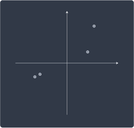
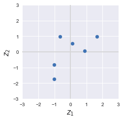
Consider the following two-dimensional dataset:

	$x_1$	$x_2$
1	9	7
2	7	5
3	3	7
4	5	6
5	2	3
6	2	1

Let's begin with a quick visualization of our dataset:

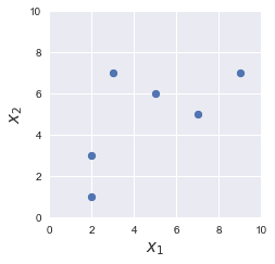
Our goal is to use PCA to reduce the dimensions of our dataset from two to one, that is, from $\mathbb{R}^2$ to $\mathbb{R}$.

Standardization

As we shall see later, PCA uses the variance of each feature to extract information, which means that the units (or magnitudes) of the features will heavily affect the outcome of PCA. For instance, suppose we want to perform PCA on two variables - a person's age and weight. If the unit of weight is in grams, then the magnitude of its spread will be much larger than that of the age variable. The variance of the weight would be in the order of magnitude of 10,000 while that of age would be 10. As a consequence, PCA would focus more on extracting information from variables with higher magnitudes and ignore the other variables of less magnitudes. As you can imagine, this leads to heavily biased results.

The way to overcome this is to initially perform standardization such that all the variables are transformed to the same unitless scale. There are multiple ways to scale features as discussed in our feature scaling guide, but PCA uses Z-score normalization:

$$\begin{equation}\label{eq:YkFd2kXG9RAP85CmSDE} z=\frac{x-\bar{x}}{\sigma} \end{equation}$$

Where:

$z$ is the scaled value of the feature
$x$ is the original value of the feature
$\bar{x}$ is the mean of all values of the feature
$\sigma$ is the standard deviation of all values of the feature

After performing this standardization, the transformed features would each have a mean of $0$ and a standard deviation of $1$.

As an example, let's manually standardize our first feature $\boldsymbol{x}_1$. We first need to compute the mean and the variance of this feature. We begin with the mean:

$$\begin{align*} \bar{x}_1&=\frac{1}{6}(9+7+3+5+2+2)\\ &\approx4.67 \end{align*}$$

Next, let's compute the standard deviation:

$$\begin{align*} \sigma_1&=\sqrt{\frac{1}{6}\sum^6_{i=1}(x_i-\bar{x})^2}\\ &=\sqrt{\frac{1}{6}\sum^6_{i=1}(x_i-4.67)^2}\\ &\approx2.62 \end{align*}$$

We can compute each scaled value of $\boldsymbol{x}_1$ like so:

$$\begin{align*} z^{(i)}_1&=\frac{x_1^{(i)}-\bar{x}_1}{\sigma_1}\\ &=\frac{x_1^{(i)}-4.67}{2.62} \end{align*}$$

Where:

$z^{(i)}_1$ is the scaled value of the $i$-th value in feature $\boldsymbol{x}_1$.
$x^{(i)}_1$ is the original $i$-th value in feature $\boldsymbol{x}_1$.

For example, to compute the first value:

$$\begin{align*} z^{(1)}_1&= \frac{x_1^{(1)}-4.67}{2.62}\\ &=\frac{9-4.67}{2.62}\\ &\approx1.65 \end{align*}$$

We repeat this process for the rest of the values in the feature to finally obtain the scaled feature $\boldsymbol{z}_1$. Remember that we've only standardized $\boldsymbol{x}_1$ here - we need to repeat the entire process (starting with computing the mean and standard deviation) for each feature ($\boldsymbol{x}_2$ in this case)!

Our dataset visually looks like the following after standardization:

As we can see, the layout of the points still looks similar even after standardization, and they are now centered around the origin!

Finding the principal components

What are principal components?

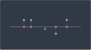
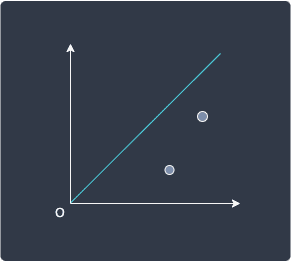
The next step of PCA is to find a line (also known as principal components) on which to project the data points that captures the relationship between the two variables well. How well the relationship is captured is based on how much variance is preserved when the points are projected onto the line. Let's intuitively understand what this means by going over a side example. Suppose we have the following data points:

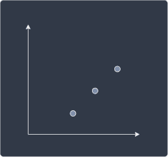
Our goal is to find a line that preserves maximal information (in the form of variance) after projection. Let's first see a line that does this horribly:

Here, we can see that the points land on the same place when they are projected onto the line. Can you see how we are losing all the information about our data points? In particular, the projected points are not spread out at all, which mathematically means that the variance of the projected points is zero. In other words, information is captured in the form of variance - the higher variance of the projected points, the more information we can capture about the variables' relationship.

In fact, this is true in other contexts of machine learning as well. If you imagine a feature having all the same values (zero variance), then that feature is useless and provides no information value when building models.

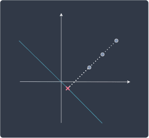
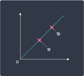
Going back to our example, let's see what a good line might like:

Here, can you see how the projected points are spread out unlike in the worse case? If we swap the original data points with the projected points, we are still preserving the underlying pattern by maintaining the variance of the original points. With this short side example, hopefully you now understand how PCA tries to minimize information loss by preserving the variance of the original data points as much as possible. The optimal line on which the data points are projected is known as principal component (PC).

How do we measure variance?

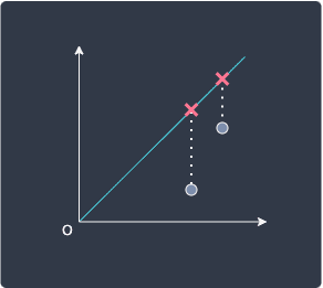
We have said that the goal of PCA is to preserve as much information as possible by maximizing the variance of the projected points. Let's make this statement mathematically precise. Straying away from our example again, suppose we had the following data points after standardization:

In PCA, we enforce a constraint that our principal component must go through the origin - you'll understand why shortly. Suppose our line and the corresponding projected points are as follows:

The objective of PCA is to maximize the variance of the projected points. To make it easier for the eyes, let's rotate the plot so that our line is horizontal:

We haven't done any transformation here - we've simply rotated the plot so that you don't have to keep tilting your head. We denote the distance between the projected data point $\boldsymbol{p}^{(i)}$ to the mean of the data points $\mu_P$ as $\Vert{\boldsymbol{p}^{(i)}}\Vert$. From elementary statistics, we know that the variance is computed as follows:

$$\begin{equation}\label{eq:SSsUkkdmek4Jc3hNEr2} \mathbb{V}(\boldsymbol{P})=\frac{1}{n}\sum^n_{i=1}(\Vert{\boldsymbol{p}^{(i)}}\Vert-\mu_P)^2 \end{equation}$$

Here, $\boldsymbol{P}$ denotes the collection of projected data points. Note that $\Vert{\boldsymbol{p}^{(i)}}\Vert$ is a scalar because it is a distance measure. Now the question is, what is the mean of the projected points $\mu_P$ in \eqref{eq:SSsUkkdmek4Jc3hNEr2}? As we will prove laterlink, the projected points are also centered around the mean! Therefore, \eqref{eq:SSsUkkdmek4Jc3hNEr2} now reduces down to the following:

$$\begin{equation}\label{eq:jZfNOtXjvJXLaEVJWiM} \mathbb{V}(\boldsymbol{P})=\frac{1}{n}\sum^n_{i=1}(\Vert{\boldsymbol{p}^{(i)}}\Vert)^2 \end{equation}$$

This is the value that PCA aims to maximize! In fact, we can actually go one step further and reduce \eqref{eq:jZfNOtXjvJXLaEVJWiM} because of the following fact:

$$\begin{equation}\label{eq:oqGRIHHLXlaS3U9KUv0} \operatorname*{argmax}_{\Vert{\boldsymbol{p}^{(i)}}\Vert} \Big(\frac{1}{n}\sum^n_{i=1}(\Vert{\boldsymbol{p}^{(i)}}\Vert)^2\Big)= \operatorname*{argmax}_{\Vert{\boldsymbol{p}^{(i)}}\Vert}\Big(\sum^n_{i=1}(\Vert{\boldsymbol{p}^{(i)}}\Vert)^2\Big) \end{equation}$$

The $\mathrm{argmax}$ just means that the maximum occurs at the same values of $\Vert{\boldsymbol{p}^{(i)}}\Vert$. Using this relationship, we conclude that PCA maximizes the following quantity:

$$\begin{equation}\label{eq:C4T2NVIe3HaVJ4P0TYd} \sum^n_{i=1}(\Vert{\boldsymbol{p}^{(i)}}\Vert)^2 \end{equation}$$

Equation \eqref{eq:C4T2NVIe3HaVJ4P0TYd} is basically the sum of squared distances from the origin to the projected data points. PCA gives us all the $\Vert{\boldsymbol{p}^{(i)}}\Vert$ that maximizes \eqref{eq:C4T2NVIe3HaVJ4P0TYd}, that is, after performing PCA, we will know the distance from the origin to each data point.

In the following section, we will go over how PCA optimizes \eqref{eq:C4T2NVIe3HaVJ4P0TYd}. Up to now, the mathematics has not been rigorous - all we've done so far is performed standardization to make each variable have a mean of zero and a standard deviation of one. The challenging part actually begins here - we need to know what variance-covariance matrices, eigenvalues and eigenvectors are in order to understand how PCA computes the optimal line. These topics are complex enough to warrant their own guides (they're coming soon by the way 🚀), so I'll only briefly discuss what they are here.

Computing the variance-covariance matrix

First, let's go over variance-covariance matrices, which fortunately are much easier to explain than eigenvalues and eigenvectors. Suppose we have two random variables $X_1$ and $X_2$. The variance-covariance matrix $\boldsymbol{\Sigma}$ of $X_1$ and $X_2$ is defined as follows:

$$\boldsymbol{\Sigma}=\begin{pmatrix} \mathbb{V}(X_1)&\mathrm{cov}(X_1,X_2)\\ \mathrm{cov}(X_2,X_1)&\mathbb{V}(X_2)\\ \end{pmatrix}$$

Where:

$X_1$ and $X_2$ are random variables
$\mathbb{V}(X_1)$ is the variance of $X_1$
$\mathrm{cov}(X_1,X_2)$ is the covariance of $X_1$ and $X_2$.

Basically, the variance-covariance matrix captures the relationship between random variables since the matrix contains the covariance of each pair of random variables.

Let's compute the variance-covariance matrix for our example:

$$\boldsymbol{\Sigma}=\begin{pmatrix} \mathbb{V}(\boldsymbol{z}_1)&\mathrm{cov}(\boldsymbol{z}_1,\boldsymbol{z}_2)\\ \mathrm{cov}(\boldsymbol{z}_2,\boldsymbol{z}_1)&\mathbb{V}(\boldsymbol{z}_2)\\ \end{pmatrix}$$

Fortunately, because we have performed standardization in the previous step, we already know what the variance of our two features is:

$$\begin{align*} \mathbb{V}(\boldsymbol{z}_1)&=1\\ \mathbb{V}(\boldsymbol{z}_2)&=1 \end{align*}$$

Next, we need to compute the covariance of $\boldsymbol{x}_1$ and $\boldsymbol{x}_2$:

$$\mathrm{cov}(\boldsymbol{z}_1,\boldsymbol{z}_2)= \frac{1}{6}\sum^6_{i=1} (z_{1}^{(i)}-\mu_1) (z_{2}^{(i)}-\mu_2)$$

Where:

$z_1^{(i)}$ is the $i$-th data of feature $\boldsymbol{x}_1$
$\mu_1$ and $\mu_2$ are the mean of $\boldsymbol{x}_1$ and $\boldsymbol{x}_2$ respectively

Once again, because we have performed standardization, we know that $\mu_1=0$ and $\mu_2=0$. Therefore, our equation reduces down to:

$$\begin{align*} \mathrm{cov}(\boldsymbol{z}_1,\boldsymbol{z}_2)&= \frac{1}{6}\sum^6_{i=1}( z_{1}^{(i)}\cdot {z_{2}^{(i)}})\\ &\approx0.63 \end{align*}$$

From the property of covariances, we know that $\mathrm{cov}(\boldsymbol{z}_1,\boldsymbol{z}_2) =\mathrm{cov}(\boldsymbol{z}_2,\boldsymbol{z}_1)$, so we don't need to calculate the latter.

With the variance and covariance computed, we now have everything we need for our variance-covariance matrix:

$$\boldsymbol{\Sigma}=\begin{pmatrix} 1&0.63\\ 0.63&1\\ \end{pmatrix}$$

Great, with the variance-covariance matrix now well defined, let's now move on to eigenvalues and eigenvectors.

NOTE

To be technically precise, the variance-covariance matrix that we computed here is actually the correlation matrix because we have standardized our data. Therefore, $\mathrm{cov}(\boldsymbol{z}_1,\boldsymbol{z}_2)$ measures the correlation instead, and the value is bound between $-1$ and $1$.

Eigenvalues and eigenvectors

Unfortunately, the concept of eigenvalues and eigenvectors is what makes PCA so difficult to understand, and the main issue is that they are abstract topics and require in-depth knowledge about linear algebra to fully grasp. I'll write a separate comprehensive guide about them very soon - join our Discord to be notified when I do - but for now, do your best to just ignore the burning question of "why?" and accept that the method works 😐.

Computing eigenvalues and eigenvectors of the variance-covariance matrix

Recall that the goal of PCA is to find the line that maximizes the variance of the projected points. It turns out that the eigenvectors of the variance-covariance matrix give us the optimal lines, or so-called principal components. I'm not going to go over the methodology behind computing eigenvalues and eigenvectors, but instead, give you the results directly. Note that I'm actually using Python's NumPy to compute these eigenvectors - please check out my Colab Notebook (Colab) for the code. The computed eigenvectors are as follows:

$$\boldsymbol{u}_1= \begin{pmatrix} 0.71\\ 0.71 \end{pmatrix} \;\;\;\;\; \boldsymbol{u}_2= \begin{pmatrix} 0.71\\ -0.71 \end{pmatrix}$$

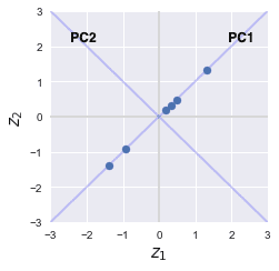
Let's plot these eigenvectors:

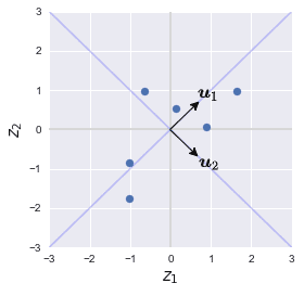
Here, note the following:

$\boldsymbol{u}_1$ and $\boldsymbol{u}_2$ are the eigenvectors of the variance-covariance matrix, and they actually maximize the variance of the projected data points.
$\boldsymbol{u}_1$ and $\boldsymbol{u}_2$ are called principal components (PCs).
the eigenvectors are always orthogonal (perpendicular) to each other.
$\boldsymbol{u}_1$ and $\boldsymbol{u}_2$ are unit-vectors, that is, they have length one.
the blue lines represent the lines onto which the data points will be projected

NOTE

If you standardize the data as we have done, then you will always get the same pair of eigenvectors as above regardless of your initial two-dimensional dataset. These eigenvectors go through the origin at 45 degrees.

From the above plot, we can see that we have two principal components. We now need to pick which principal component we want to project our data points to. The decision is never made randomly since the individual principal components retain varying amounts of information of the original data points. In order to pick the best principal components that preserve the most information of the original data points, we check the corresponding eigenvalues of the eigenvectors. For each eigenvector, there exists a corresponding eigenvalue, and hence in our case, we have 2 eigenvalues to check. These eigenvalues are extremely important because they tell us how much information is preserved - the higher the eigenvalue, the more information that is preserved. In this case, the eigenvalues of $\boldsymbol{u}_1$ and $\boldsymbol{u}_2$ are computed as follows:

$$\begin{align*} \lambda_1&=1.63\\ \lambda_2&=0.37 \end{align*}$$

Where:

$\lambda_1$ is the eigenvalue of the eigenvector $\boldsymbol{u}_1$
$\lambda_2$ is the eigenvalue of the eigenvector $\boldsymbol{u}_2$

We can see that the eigenvalue of $\boldsymbol{u}_1$ is greater than that of $\boldsymbol{u}_2$. This means that the principal component $\boldsymbol{u}_1$ preserves more information than $\boldsymbol{u}_2$, and hence we should pick $\boldsymbol{u}_1$ to project our data points onto. The eigenvector with the highest eigenvalue is called the 1st principal component (PC1), and the eigenvector with the second-highest eigenvalue is called the 2nd principal component (PC2), and so on. In this case, $\boldsymbol{u}_1$ is PC1 and $\boldsymbol{u}_2$ is PC2.

Computing the explained variance ratio

We have just discussed how eigenvalues give us an idea of how much information their corresponding eigenvector contains if we were to project our data points onto them. Instead of comparing eigenvalues directly, we often compute a simple measure called explained variance ratio like so:

$$r_i=\frac{\lambda_i}{\sum^m_{j=1}\lambda_j}$$

Where:

$r_i$ is the explained variance of the $i$-th eigenvector
$\lambda_i$ is the eigenvalue of the $i$-th eigenvector
$m$ is the number of eigenvectors

In our example, we only have two eigenvalues ($m=2$), and so we just need to compute two explained variance ratios like so:

$$\begin{align*} r_1&=\frac{\lambda_1}{\lambda_1+\lambda_2}=\frac{1.63}{1.63+0.37}\approx0.81\\ r_2&=\frac{\lambda_2}{\lambda_1+\lambda_2}=\frac{0.37}{1.63+0.37}\approx0.19 \end{align*}$$

We usually plot a simple bar graph of the explained variance ratios:

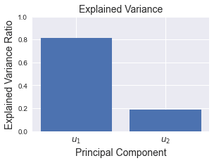
As you can see, the explained variance ratio for $\boldsymbol{u}_1$ is much greater than $\boldsymbol{u}_2$, which is what we should expect since the eigenvalue of $\boldsymbol{u}_1$ is much larger than $\boldsymbol{u}_2$. The reason why explained variance ratio is typically computed instead of directly comparing eigenvalues is that the value of the explained variance ratio of a principal component can be interpreted as how much of the information is preserved if we were to project our points onto that principal component. For instance, if we project our dataset onto the PC1 ($\boldsymbol{u}_1$), then we would be able to preserve roughly 81% of the original information - which is quite good!

Projecting data points onto principal components

So far, we have computed the principal components and their explained variance ratios. Since the explained variance ratio of $\boldsymbol{u}_1$ is greater than that of $\boldsymbol{u}_2$, we will project our points to $\boldsymbol{u}_1$ instead of $\boldsymbol{u}_2$. We now need to project our data points onto the principal components to perform dimensionality reduction. Note that we are not specifically after the coordinates of the projected points, but instead we are after the distance from the origin to each projected point, that is, $\Vert{\boldsymbol{p}^{(i)}}\Vert$.

Computing projection lengths

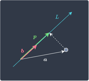
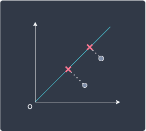
In order to obtain the distance from the origin to each projected point, we can turn to linear algebra. Let's forget our example for a quick moment, and review the concept of projections in linear algebra. Consider the following diagram:

Here, $\boldsymbol{p}$ is the vector that results from an orthogonal projection from point $\boldsymbol{a}$ to the line $L$. The vector $\boldsymbol{b}$ is any vector that points in the same direction as the line $L$. The dot product of two vectors $\boldsymbol{a}$ and $\boldsymbol{b}$returns the following:

$$\begin{equation}\label{eq:jgRja3ct84jO5INXSY2} \boldsymbol{a}\cdot\boldsymbol{b}=\Vert{\boldsymbol{p}}\Vert\Vert{\boldsymbol{b}}\Vert \end{equation}$$

Where $\Vert{\boldsymbol{p}}\Vert$ and $\Vert\boldsymbol{b}\Vert$ are the lengths of vectors $\boldsymbol{p}$ and $\boldsymbol{b}$ respectively.

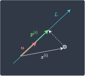
Let's now change the notations to align with our example:

Here,

$\boldsymbol{u}_1$ is our PC1 - a unit-eigenvector of length one
$\boldsymbol{z}^{(i)}$ is the $i$-th scaled observation
$\boldsymbol{p}^{(i)}_1$ is the vector resulting from the orthogonal projection on PC1

Using the logic of \eqref{eq:jgRja3ct84jO5INXSY2}, the dot product of $\boldsymbol{u}_1$ and $\boldsymbol{z}^{(i)}$ is:

$$\boldsymbol{u}_1\cdot\boldsymbol{z}^{(i)}=\Vert{\boldsymbol{p}_1^{(i)}}\Vert\Vert{\boldsymbol{u}_1}\Vert$$

Since $\boldsymbol{u}_1$ is a unit vector of length one, this formula reduces down to the following:

$$\begin{equation}\label{eq:JMuMdacxJ2m0j4VvwX1} \boldsymbol{u}_1\cdot\boldsymbol{z}^{(i)}=\Vert{\boldsymbol{p}^{(i)}_1}\Vert \end{equation}$$

This means that in order to obtain the length from the origin to the projected point, we just need to take the dot product between our eigenvector (PC1) and each data point - simple!

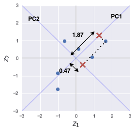
Going back to our example, let's try computing $\Vert{\boldsymbol{p}^{(1)}_1}\Vert$ for the right-most data point $\boldsymbol{z}^{(1)}$, which is represented by the following coordinate vector:

$$\boldsymbol{z}^{(1)}= \begin{pmatrix} 1.65\\ 0.99\\ \end{pmatrix}$$

Using \eqref{eq:JMuMdacxJ2m0j4VvwX1}, let's compute $\Vert{\boldsymbol{p}^{(1)}_1}\Vert$:

$$\begin{align*} \Vert{\boldsymbol{p}^{(1)}_1}\Vert&=\boldsymbol{u}_1\cdot\boldsymbol{z}^{(1)}\\ &= \begin{pmatrix} 0.71\\ 0.71\\ \end{pmatrix} \cdot \begin{pmatrix} 1.65\\ 0.99\\ \end{pmatrix} \\ &\approx 1.87 \end{align*}$$

This means that the length from the origin to the first projected point is $1.87$.

Now, we need to perform the same step for each of the other data points. Mathematically, we can neatly represent this operation with the help of matrices. Let's pack our eigenvectors into a single matrix, which we call $\boldsymbol{W}$:

$$\boldsymbol{W}= \begin{pmatrix} \vert&\vert\\ \boldsymbol{u}_1&\boldsymbol{u}_2\\ \vert&\vert \end{pmatrix}$$

Here, the eigenvectors are stacked horizontally. In our case, the content of $\boldsymbol{W}$ would be:

$$\boldsymbol{W}= \begin{pmatrix} 0.71&0.71\\ 0.71&-0.71 \end{pmatrix}$$

Similarly, let's also pack our data points into a single matrix $\boldsymbol{Z}$:

$$\boldsymbol{Z}= \begin{pmatrix} -&\boldsymbol{z}^{(1)}&-\\ -&\boldsymbol{z}^{(2)}&-\\ -&\vdots&-\\ -&\boldsymbol{z}^{(6)}&-\\ \end{pmatrix}$$

In our example, each row of $\boldsymbol{Z}$ represents a data point that lives in $\mathbb{R}^2$. This means that $\boldsymbol{Z}\in\mathbb{R}^{6\times2}$, that is, $\boldsymbol{Z}$ has $6$ rows and $2$ columns. Let's now compute the product of $\boldsymbol{Z}$ and $\boldsymbol{W}$, which we will call $\boldsymbol{X}'$:

$$\begin{align*} \boldsymbol{X}'&=\boldsymbol{Z}\boldsymbol{W}\\ &=\begin{pmatrix} -&\boldsymbol{z}^{(1)}&-\\ -&\boldsymbol{z}^{(2)}&-\\ -&\vdots&-\\ -&\boldsymbol{z}^{(6)}&-\\ \end{pmatrix} \begin{pmatrix} \vert&\vert\\ \boldsymbol{u}_1&\boldsymbol{u}_2\\ \vert&\vert \end{pmatrix}\\ &= \begin{pmatrix} \boldsymbol{z}^{(1)}\cdot{\boldsymbol{u}}_1& \boldsymbol{z}^{(1)}\cdot{\boldsymbol{u}}_2\\ \boldsymbol{z}^{(2)}\cdot{\boldsymbol{u}}_1& \boldsymbol{z}^{(2)}\cdot{\boldsymbol{u}}_2\\ \vdots&\vdots\\ \boldsymbol{z}^{(6)}\cdot{\boldsymbol{u}}_1& \boldsymbol{z}^{(6)}\cdot{\boldsymbol{u}}_2 \end{pmatrix}\\ &= \begin{pmatrix} \Vert\boldsymbol{p}^{(1)}_1\Vert&\Vert\boldsymbol{p}^{(1)}_2\Vert\\ \Vert\boldsymbol{p}^{(2)}_1\Vert&\Vert\boldsymbol{p}^{(2)}_2\Vert\\ \vdots&\vdots\\ \Vert\boldsymbol{p}^{(6)}_1\Vert&\Vert\boldsymbol{p}^{(6)}_2\Vert \end{pmatrix} \end{align*}$$

Since $\boldsymbol{Z}\in\mathbb{R}^{6\times2}$ and $\boldsymbol{W}\in\mathbb{R}^{2\times2}$, the resulting dimensions of $\boldsymbol{X}'$ would be $\mathbb{R}^{6\times2}$. Here, $\boldsymbol{X}'$ holds $\Vert\boldsymbol{p}^{(i)}_1\Vert$ and $\Vert\boldsymbol{p}^{(i)}_2\Vert$, which represent the lengths from the origin to the projected data points on both PC1 (first column) and PC2 (second column) respectively. Since we know that PC1 preserves much more information than PC2, we can choose to ignore PC2 (second column). Computationally, this is useful because we can actually set $\boldsymbol{W}$ to hold just the first principal component, thereby saving computation time and memory.

Great, we have now managed to obtain a general formula to compute the length from the origin to each projected data point for both principal components!

Let's now compute $\boldsymbol{X}'$ in our example, which simply requires computing the dot product of every pair of $\boldsymbol{z}^{(i)}$ and the two eigenvectors $\boldsymbol{u}_1$ and $\boldsymbol{u}_2$. Here are the results:

$$\boldsymbol{X}'= \begin{pmatrix} 1.87&-0.47\\ 0.68&-0.57\\ 0.25&1.15\\ 0.47&0.29\\ -1.31&0.13\\ -1.95&-0.52\\ \end{pmatrix}$$

Let's summarize our final results in a table:

	$x'_1$ (PC1)	$x'_2$ (PC2)
1	1.87	-0.47
2	0.68	-0.57
3	0.25	1.15
4	0.47	0.29
5	-1.31	0.13
6	-1.95	-0.52

Here:

$x'_1$ represents the length from the origin to the projected point on PC1 ($\Vert\boldsymbol{p}^{(i)}_1\Vert$)
$x'_2$ represents the length from the origin to the projected point on PC2 ($\Vert\boldsymbol{p}^{(i)}_2\Vert$)

For example, the following diagram illustrates what the values represent for the first data point:

Projecting onto PC1

We now select PC1 to project our data points onto. We plot $x'_1$ on a number line:

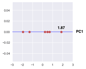
These one-dimensional values retain the most amount of information (captured through variance) of the original two-dimensional data points! The final transformed data points in tabular form are as follows:

	$x'_1$ (PC1)
1	1.87
2	0.68
3	0.25
4	0.47
5	-1.31
6	-1.95

We're actually now done with our task of performing dimensionality reduction! The rest of the guide will cover other aspects of PCA in more detail.

Projecting onto PC2

We could also perform dimensionality reduction by selecting PC2 instead of PC1:

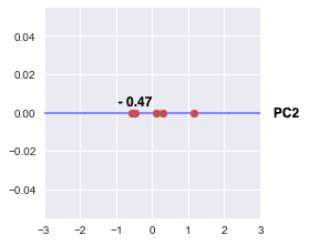
Notice how, compared to PC1, the variance of the projected points on PC2 is low. This means that projecting onto PC1 is much more desirable than onto PC2 as PC1 preserves more information with a smaller variance loss. This is to be expected because the explained variance ratio of PC1 is much greater than PC2 as discussed in the previous sectionlink.

Projecting onto both PC1 and PC2

We have just looked at how we can perform dimensionality reduction by projecting our data points onto a single principal component. We could, however, project our data points onto both the principal components, in which case, the number of dimensions of the resulting projected data points would still remain as 2.

Recall that the projected point on both PC1 and PC2 for the first data point was as follows:

If we select both PC1 and PC2 to perform projection, the transformed points would be as follows:

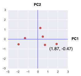
Here, we have rotated our previous plot 45 degrees to make PC1 and PC2 the axes line of a new coordinate system! The transformed coordinate of the first data point in this new coordinate system is $(1.87, -0.47)$.

Interpreting eigenvectors as weights of features

Recall that in order to compute the new coordinates, we took the dot product of an eigenvector $\boldsymbol{u}$ and the standardized data point $\boldsymbol{z}^{(i)}$. For instance, to compute the new coordinate of the $i$-th data point with PC1 as the axis line:

$$\begin{align*} \Vert{\boldsymbol{p}^{(i)}_1}\Vert&=\boldsymbol{u}_1\cdot{\boldsymbol{z}^{(i)}}\\ &=u_1^{(1)}z_1^{(i)}+u_1^{(2)}z_2^{(i)}\\ \end{align*}$$

Here, $u_1^{(1)}\in\mathbb{R}$ and $u_1^{(2)}\in\mathbb{R}$ are the first and second elements of the eigenvector $\boldsymbol{u}_1$. In linear algebra, we call the above a linear combination of variables and you can interpret $u_1^{(1)}$ and $u_1^{(2)}$ as the weights (or importance) assigned to each dimension (or feature) of the data point $\boldsymbol{z}^{(i)}$. For instance, if the value of $u_1^{(2)}$ is high, then this means that the second feature of $\boldsymbol{z}^{(i)}$ has a large impact on the resulting projection. In our example, $u_1^{(1)}=u_1^{(2)}=0.71$, so the weighting of each feature of $\boldsymbol{z}^{(i)}$ is the same. However, as we shall see in the latter section on performing PCA on the Iris datasetlink, these weights help us to make sense of the meaning behind principal components.

Reconstructing the original data points

Mathematical theory

Recall that we have performed the following transformation to obtain the length from the origin to the projected point for the principal components:

$$\boldsymbol{X}'=\boldsymbol{Z}\boldsymbol{W}$$

In order to obtain the original standardized dataset $\boldsymbol{Z}$ back, we just need to rewrite the above as follows:

$$\begin{equation}\label{eq:qcrQxvjUQeb9VeqAPNl} \boldsymbol{Z}=\boldsymbol{X}'\boldsymbol{W}^{-1} \end{equation}$$

Where $\boldsymbol{W}^{-1}$ is the inverse matrix of $\boldsymbol{W}$. Interestingly, $\boldsymbol{W}$ here is an orthogonal matrix, which is basically a matrix where:

each vector (represented by columns of the matrix) is perpendicular to each other
every vector is a unit-vector of length one.

Recall that the columns of $\boldsymbol{W}$ are made up of eigenvectors:

$$\boldsymbol{W}= \begin{pmatrix} \vert&\vert\\ \boldsymbol{u}_1&\boldsymbol{u}_2\\ \vert&\vert \end{pmatrix}$$

From the visual plot of the two eigenvectors, we know that they are perpendicular to each other. Moreover, we have said that the eigenvectors are already converted into a unit-vector such that their lengths are one. Since both conditions are satisfied, $\boldsymbol{W}$ is considered as an orthogonal matrix. The reason this is important to us is that, orthogonal matrices exhibit the following property:

$$\boldsymbol{W}^{-1}=\boldsymbol{W}^T$$

This means that the inverse of $\boldsymbol{W}$ is equal to the transpose of $\boldsymbol{W}$. With this, we can rewrite \eqref{eq:qcrQxvjUQeb9VeqAPNl} as follows:

$$\begin{equation}\label{eq:KiJf8JY7PHXp9aHSOMG} \boldsymbol{Z}=\boldsymbol{X}'\boldsymbol{W}^{T} \end{equation}$$

This reformulation is useful because computing the transpose, which involves just swapping the rows and columns, is much easier than computing the inverse of a matrix.

Reconstructing the original data points for our example

In this section, in order to demonstrate information loss that happens after PCA, we will go over what the reconstructed original points would look like after the following two scenarios:

selecting all principal components (using PC1 and PC2 in our case)
reducing the dimension by only using a subset of principal components (using PC1 and ignoring PC2 in our case)

Using both PC1 and PC2

We have said that there is no information loss in the first scenario in which we select all the principal components. This would mean that we will be able to exactly reconstruct the original data points using the transformed points.

Let's demonstrate this using our example. Recall that our transformed data points after PCA was as follows:

$$\boldsymbol{X}'= \begin{pmatrix} 1.87&-0.47\\ 0.68&-0.57\\ 0.25&1.15\\ 0.47&0.29\\ -1.31&0.13\\ -1.95&-0.52\\ \end{pmatrix}$$

Remember that $\boldsymbol{W}$ is a matrix where the columns are the eigenvectors. The transpose of $\boldsymbol{W}$ therefore has rows as the eigenvectors:

$$\begin{align*} \boldsymbol{W}^T&= \begin{pmatrix} -&\boldsymbol{u}_1&-\\ -&\boldsymbol{u}_2&-\\ \end{pmatrix}\\ &= \begin{pmatrix} 0.71&0.71\\ 0.71&-0.71\\ \end{pmatrix} \end{align*}$$

Using equation \eqref{eq:KiJf8JY7PHXp9aHSOMG}, we can obtain the original standardized data points:

$$\begin{align*} \boldsymbol{Z} &=\boldsymbol{X}'\boldsymbol{W}^{T}\\ &\approx \begin{pmatrix} 1.87&-0.47\\ 0.68&-0.57\\ 0.25&1.15\\ 0.47&0.29\\ -1.31&0.13\\ -1.95&-0.52\\ \end{pmatrix} \end{align*} $$

Each row of $\boldsymbol{Z}$ represents the coordinate of the original standardized data points. Let's plot them to confirm we indeed return to the data points before the projection:

Original points	Recomputed points

Great, the original and recomputed points are exactly identical! We can actually explain this behavior by referring to the explained variance ratio. We show the explained variance ratio plot here again for your reference:

As a reminder, we can interpret the explained variance ratio of a principal component as the percentage of information that the principal component preserves. So for example, the first principal component captures roughly 80% of the information contained in the original data point. The explained variance ratios will always add up to one, and so if we select both PC1 and PC2, then the total explained variance ratio would equal 100%, which means that there is no information loss!

NOTE

In the context of machine learning, PCA is more often used for dimensionality reduction rather than remapping the data points in a new coordinate system as we have done in this section.

Using only PC1

Let us now look at the second scenario where we select only PC1. Since we ignore PC2, we can discard the second column of $\boldsymbol{X}'$, so $\boldsymbol{X}'$ would look like the following:

$$\boldsymbol{X}'= \begin{pmatrix} 1.87\\ 0.68\\ 0.25\\ 0.47\\ -1.31\\ -1.95\\ \end{pmatrix}$$

Similarly, we can ignore the second eigenvector of $\boldsymbol{W}^T$, which represents PC2. Therefore $\boldsymbol{W}^T$ would contain only the first eigenvector:

$$\begin{align*} \boldsymbol{W}^T&= \begin{pmatrix} -&\boldsymbol{u}_1&- \end{pmatrix}\\ &= \begin{pmatrix} 0.71&0.71 \end{pmatrix} \end{align*}$$

Here, $\boldsymbol{X}'\in\mathbb{R}^{6\times1}$ and $\boldsymbol{W}^T\in\mathbb{R}^{1\times2}$ so $\boldsymbol{Z}\in\mathbb{R}^{6\times2}$, as we see below:

$$\begin{align*} \boldsymbol{Z} &=\boldsymbol{X}'\boldsymbol{W}^{T}\\ &\approx \begin{pmatrix} 1.32&1.32\\ 0.48&0.48\\ 0.18&0.18\\ 0.33&0.33\\ -0.93&-0.93\\ -1.38&-1.38\\ \end{pmatrix} \end{align*} $$

Let's plot $\boldsymbol{Z}$ to visualize the retrieved data points:

Original points	Recomputed points

Can you see how the recomputed data points have retained their variation along PC1 but now ignores the variation along PC2? It is impossible to reconstruct the original data points if we only select a subset of principal components because some information will be inevitably lost during dimensionality reduction. In fact, we can quantify how much information is lost using the concept of explained variance ratio again:

By only using PC1, we preserve 80% of the information contained in the original data points!

NOTE

In order to retrieve the original data points back before standardization, we can simply rearrange formula \eqref{eq:vgKhK1G7HFMsCuP90sf} for standardization to make $x$ the subject:

$$x^{(i)}_j=z^{(i)}_j\sigma_j+\bar{x}_j$$

Where:

$x^{(i)}_j$ is the $i$-th original data point in feature $j$
$z^{(i)}_j$ is the $i$-th scaled data point in feature $j$
$\sigma_j$ is the standard deviation of the original values in feature $j$
$\bar{x}_j$ is the mean of the original values in feature $j$

Supplementary information about PCA

Mathematical proof that the projected points are centered around the origin

Recall that the variance of the projected points $\boldsymbol{P}$ is computed like so:

$$\mathbb{V}(\boldsymbol{P})=\frac{1}{n}\sum^n_{i=1}(\Vert{\boldsymbol{p}^{(i)}}\Vert-\mu_P)^2$$

Where:

$n$ is the number of data points
$\Vert{\boldsymbol{p}^{(i)}}\Vert$ is the length from the origin to the projected point $\boldsymbol{p}^{(i)}$
$\mu_p$ is the mean of the projected points

We have claimed in the previous sectionlink that, just like the standardized points, the projected points are also centered around the origin. Therefore, the above equation can be reduced to the following:

$$\mathbb{V}(\boldsymbol{P})=\frac{1}{n}\sum^n_{i=1}(\Vert{\boldsymbol{p}^{(i)}}\Vert)^2$$

In this section, we will prove this claim.

Firstly, we've standardized our dataset in the first step such that the mean of every feature is zero:

$$\begin{equation}\label{eq:dD1s6SNotyWBa3KxOaq} \frac{1}{n}\sum^n_{i=1}z^{(i)}_j=0\;\;\;\Rightarrow\;\;\;\sum^n_{i=1}z^{(i)}_j=0 \end{equation}$$

Using \eqref{eq:dD1s6SNotyWBa3KxOaq}, let us prove that the mean vector $\boldsymbol{\mu}_P$ of the projected points $\boldsymbol{p}^{(i)}$ is actually just the origin:

$$\begin{align} \boldsymbol{\mu}_P&=\frac{1}{n}\sum^n_{i=1}\boldsymbol{p}^{(i)}\tag{$\star1$}\\ &=\frac{1}{n}\sum^n_{i=1}(\boldsymbol{z}^{(i)}\cdot{\boldsymbol{u}})\boldsymbol{u}\tag{$\star2$}\\ &=\frac{1}{n}\Big[(\boldsymbol{z}^{(1)}\cdot{\boldsymbol{u}})\boldsymbol{u} +(\boldsymbol{z}^{(2)}\cdot{\boldsymbol{u}})\boldsymbol{u} +\cdots +(\boldsymbol{z}^{(n)}\cdot{\boldsymbol{u}})\boldsymbol{u}\Big]\tag{$\star3$} \\ &=\frac{1}{n}\Big[ (\boldsymbol{z}^{(1)}\cdot{\boldsymbol{u}} +\boldsymbol{z}^{(2)}\cdot{\boldsymbol{u}} +\cdots +\boldsymbol{z}^{(n)}\cdot{\boldsymbol{u}})\Big] \boldsymbol{u}\tag{$\star4$}\\ &=\frac{1}{n}\Big[ \Big(\sum^{n}_{i=1}z^{(i)}_1\Big)u_1 +\Big(\sum^{n}_{i=1}z^{(i)}_2\Big)u_2 +\cdots +\Big(\sum^{n}_{i=1}z^{(i)}_m\Big)u_m \Big] \boldsymbol{u}\tag{$\star5$}\\ &=\frac{1}{n}\Big[ 0 +0 +\cdots +0 \Big]\boldsymbol{u}\tag{$\star6$} \\ &=\boldsymbol{0}\tag{$\star7$} \end{align}$$

Here, to get from step $\star{1}$ to step $\star2$, we used the definition of projections in linear algebra. Let's quickly review the topic of projections here.

Consider the following setup:

Here, we are projecting the data point represented by position vector $\boldsymbol{a}$ onto the line $L$. The projected point is denoted by position vector $\boldsymbol{p}$, and vector $\boldsymbol{b}$ is some vector that points in the same direction as line $L$. Linear algebra relates these vectors with the following formula:

$$\begin{equation}\label{eq:TLkufj9nRwFW04NjdMi} \boldsymbol{p}=(\boldsymbol{a}\cdot{\boldsymbol{b}})\boldsymbol{b} \end{equation}$$

To align with our example, let's change the syntax:

Using the same logic as \eqref{eq:TLkufj9nRwFW04NjdMi}, we know that the following relationship holds:

$$\boldsymbol{p}^{(i)}=(\boldsymbol{z}^{(i)}\cdot{\boldsymbol{u}})\boldsymbol{u}$$

This is how we get from step $\star1$ to step $\star2$.

Reframing PCA as an optimization problem to minimize projection distance

Some guides may frame PCA as an optimization problem where we minimize the sum of the perpendicular distance from each point to the projection line, which is in contrast to how I framed PCA as an optimization problem to maximize the variance of the projected data points. In this section, we will prove that these two formulations are actually equivalent.

Consider the following data points:

For the former optimization problem of minimizing the sum of the perpendicular distance to the projection line from each point, we are trying to minimize the length of the following dotted lines:

Let's now reframe this optimization using our old friend, Pythagoras theorem. Let's focus on the bottom-left data point:

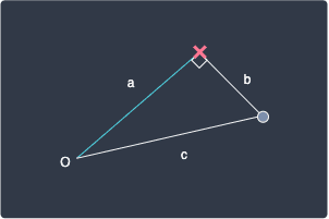
Here, $b$ is the perpendicular distance from the point to the line, $a$ is the distance from the origin to the projected point on the line, and $c$ is the hypotenuse. Pythagoras theorem tells us that:

$$c^2=a^2+b^2$$

Since we are trying to minimize $b$, let's make it the subject:

$$b=\sqrt{c^2-a^2}$$

The $c$ here is a constant because the distance between the origin and the data point never changes. This means that we can actually minimize $b$ by maximizing $a$! In other words, we can equivalently maximize the distance from the origin to the projected point on the line, which is essentially equation \eqref{eq:C4T2NVIe3HaVJ4P0TYd}:

$$\sum^n_{i=1}(\Vert{\boldsymbol{z}^{(i)}}\Vert)^2$$

Where $\Vert{\boldsymbol{z}^{(i)}}\Vert$ is the distance between the origin and the standardized data point $\boldsymbol{z}^{(i)}$. As we have derived in the earlier sectionlink, maximizing the above equation is also equivalent to maximizing the variance of the projected points!

Connection to linear regression

The optimization problem of minimizing the sum of projection distances may remind you of linear regression, where we try to find a line of best fit through the data points. However, how we determine the optimal line is not the same - in regression, we minimize the residual which is defined by the vertical distance from the data point to the line:

However, PCA determines the "best" line by minimizing the perpendicular distance to the line:

Performing PCA on real-world datasets using Python's Scikit-learn

Colab Notebook for Principal Component Analysis (PCA)

Please log in or sign up to access the colab notebook

Click here to access all the Python code snippets used for this guide!

lock

Using PCA to reduce the number of features

Let's perform PCA using Python's Scikit-learn library on a real dataset - the classic Iris dataset - to demonstrate dimensionality reduction.

Importing dataset

We begin by importing the Iris dataset:


        
        
            
                
                
                    import numpy as np
import pandas as pd

df_raw = pd.read_csv('https://raw.githubusercontent.com/SkyTowner/sample_data/main/iris_dataset')
df_raw.head()
                
            
               sepal_length  sepal_width  petal_length  petal_width  species
0      5.1           3.5          1.4           0.2      setosa
1      4.9           3.0          1.4           0.2      setosa
2      4.7           3.2          1.3           0.2      setosa
3      4.6           3.1          1.5           0.2      setosa
4      5.0           3.6          1.4           0.2      setosa

Here, the first 4 columns are our features and the target is the species column. Since the goal is to reduce the feature space, we can ignore the species column. Let's reduce our feature space from $\mathbb{R}^4$ to $\mathbb{R}^2$ so that we can visualize our features using a two-dimensional scatter plot.

Firstly, let's first create another DataFrame without the target label species:


        
        
            
                
                
                    df_X = df_raw.drop(columns='species')
df_X.head()
                
            
               sepal_length  sepal_width  petal_length  petal_width  species
0      5.1           3.5          1.4           0.2      setosa
1      4.9           3.0          1.4           0.2      setosa
2      4.7           3.2          1.3           0.2      setosa
3      4.6           3.1          1.5           0.2      setosa
4      5.0           3.6          1.4           0.2      setosa

Note that drop(~) creates a new DataFrame and leaves the original one intact.

Standardizing the dataset

The first step of PCA is standardization in which we transform each feature such that its mean and standard deviation become 0 and 1 respectively. We can do this easily using Scikit-learn's StandardScalar library:


        
        
            
                
                
                    from sklearn.preprocessing import StandardScaler

sc = StandardScaler()
scaled_X = sc.fit_transform(df_X)   # Returns a NumPy array
scaled_X[:5]   # Show the first 5 rows
                
            
            array([[-0.90068117,  1.03205722, -1.3412724 , -1.31297673],
       [-1.14301691, -0.1249576 , -1.3412724 , -1.31297673],
       [-1.38535265,  0.33784833, -1.39813811, -1.31297673],
       [-1.50652052,  0.10644536, -1.2844067 , -1.31297673],
       [-1.02184904,  1.26346019, -1.3412724 , -1.31297673]])

Great, each row represents a data point, and each column has a mean of zero and a standard deviation of one!

Dimensionality reduction using PCA

With the data points now standardized, let's perform PCA. This is extremely easy and can be done in two lines:


        
        
            
                
                
                    from sklearn.decomposition import PCA

pca = PCA(n_components=2)
X_pca = pca.fit_transform(scaled_X)   # Returns a NumPy array 
X_pca[:5]
                
            
            array([[-2.26454173,  0.5057039 ],
       [-2.0864255 , -0.65540473],
       [-2.36795045, -0.31847731],
       [-2.30419716, -0.57536771],
       [-2.38877749,  0.6747674 ]])

Here, we have specified that n_components=2, which means that we want to use the first and second principal components.

To obtain the values for PC1 (first column) and PC2 (second column), we can use NumPy's indexing:


        
        
            
                
                
                    PC1 = X_pca[:,0]   # Extract the first column
PC2 = X_pca[:,1]   # Extract the second column

NOTE

PCA is a deterministic algorithm, that is, no matter how many times you run PCA, we will always get the same results. There is no randomness involved!

Let's pack PC1 and PC2 as well as their corresponding labels in a Pandas DataFrame:


        
        
            
                
                
                    df = pd.DataFrame({'PC1': PC1, 'PC2': PC2, 'label': df_raw['species']})
df.head()
                
            
               PC1        PC2        label
0  -2.264542  0.505704   setosa
1  -2.086426  -0.655405  setosa
2  -2.367950  -0.318477  setosa
3  -2.304197  -0.575368  setosa
4  -2.388777  0.674767   setosa

Let's use seaborn to plot a scatterplot of PC1 and PC2 along with their corresponding labels:


        
        
            
                
                
                    import seaborn as sns
import matplotlib.pyplot as plt

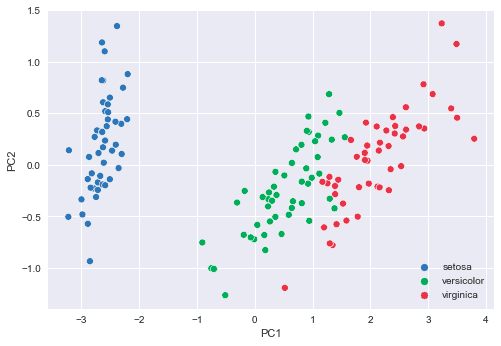
sns.scatterplot(data=df, x="PC1", y="PC2", hue="label")
plt.xlabel('PC1', fontsize=14)
plt.ylabel('PC2', fontsize=14)
plt.legend(fontsize=13, title_fontsize='40')
plt.show()

This returns the following plot:

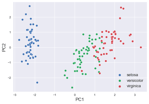
We can see that PC1 and PC2 separate the 3 species of Iris well. This means that PCA has managed to preserve most of the information when reducing the original four-dimensional data points into just two dimensions. Note that even though we show the labels here, PCA is an unsupervised learning algorithm and makes no use of the labels during training.

You can obtain the eigenvectors - the principal components - through the components_ property:


        
        
            
                
                
                    pca.components_
                
            
            array([[ 0.52237162, -0.26335492,  0.58125401,  0.56561105],
       [ 0.37231836,  0.92555649,  0.02109478,  0.06541577]])

Here, we have 2 components because we have specified n_components=2.

We can also access the explained variance ratio of our PCA:


        
        
            
                
                
                    pca.explained_variance_ratio_
                
            
            array([0.72770452, 0.23030523])

We see that the first principal component holds roughly 73% of the information, while the second principal component contains nearly 23% of the information. Remember, information is captured through the form of variance.

In total, the two principal components explain roughly 96% of original features:


        
        
            
                
                
                    np.sum(pca.explained_variance_ratio_)
                
            
            0.9580097536148198

This is to be expected after seeing our scatter plot because we already know that the PC1 and PC2 capture information that can differentiate the 3 species of Iris very well.

Interpreting the components

Recall that we can interpret the components as the weight placed on each feature value:


        
        
            
                
                
                    for index, component in enumerate(np.round(pca.components_, 2)):
    res = []
    for value, col_name in zip(component, df_X.columns):
        res.append(f'{value} {col_name}')
    print(f'PC{index+1}: ' + ' + '.join(res))
                
            
            PC1: 0.52 sepal_length + -0.26 sepal_width + 0.58 petal_length + 0.57 petal_width
PC2: 0.37 sepal_length + 0.93 sepal_width + 0.02 petal_length + 0.07 petal_width

Here, we can see that the petal_length is the most important factor in determining the projected value on PC1, whereas the sepal_width is by far the most important factor in PC2.

Using PCA to reduce the dimensions of images

This section and the following sections are heavily inspired by the excellent book "Python Data Science Handbook"open_in_new, so credits go to the author of the book. A portion of the code here is adapted from the book's code, which is released under MIT license.

Images are tricky to handle in machine learning because they exist in a high-dimensional space. For instance, a small 32 by 32 pixel image holds $32\times32=1024$ values in total, which means that this small image actually resides in $\mathbb{R}^{1024}$. This makes dimensionality reduction techniques such as PCA extremely useful in processing images!

In this section, let's use PCA to visualize images of numerical digits on a single scatterplot. The dataset we will use is the classic MNIST handwritten digits provided by Sklearn. Let's first import the dataset:


        
        
            
                
                
                    from sklearn.datasets import load_digits

digits = load_digits()
digits.data.shape
                
            
            (1797, 64)

Unlike the official MNIST dataset, which has 70,000 images of 28 by 28 pixel handwritten digits, Sklearn's version is much smaller with only 1797 images of 8 by 8 pixel handwritten digits. The reason why we see 64 in the shape above is that the images are not expressed by a two-dimensional array but by a one-dimensional flat array.

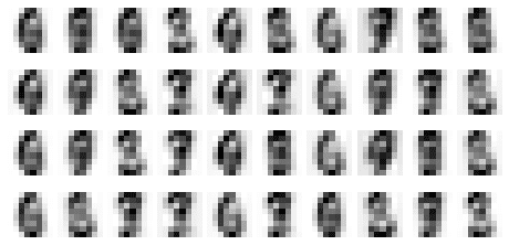
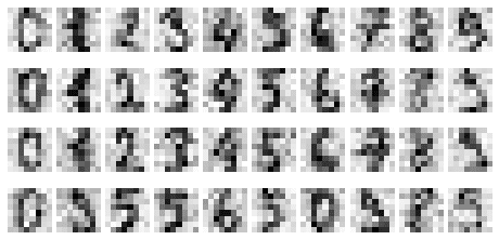
In order to visualize the digits, let's first define a helper function that plots 4 sets of digits from 0 to 9:


        
        
            
                
                
                    def show_digits(data):
    # Create a 4 by 10 subplots
    # xticks:[] and yticks:[] used to remove numbered labels
    fig, axes = plt.subplots(4, 10, figsize=(8, 4),
                             subplot_kw={'xticks':[], 'yticks':[]},
                             gridspec_kw=dict(hspace=0.1, wspace=0.1))

    for i, ax in enumerate(axes.flat):
        ax.imshow(data[i].reshape(8, 8))

We can use the helper function like so:


        
        
            
                
                
                    show_digits(digits.data)

This gives us the following plot:

Just as we did for the Iris dataset, let's reduce our data points from $\mathbb{R}^{64}$ to $\mathbb{R}^2$.

The first step is to standardize each feature:


        
        
            
                
                
                    from sklearn.preprocessing import StandardScaler

sc = StandardScaler()
scaled_X = sc.fit_transform(digits.data)
scaled_X[0]
                
            
            array([ 0.        , -0.33501649, -0.04308102,  0.27407152, -0.66447751,
       -0.84412939, -0.40972392, -0.12502292, -0.05907756, -0.62400926,
        0.4829745 ,  0.75962245, -0.05842586,  1.12772113,  0.87958306,
       -0.13043338, -0.04462507,  0.11144272,  0.89588044, -0.86066632,
       -1.14964846,  0.51547187,  1.90596347, -0.11422184, -0.03337973,
        0.48648928,  0.46988512, -1.49990136, -1.61406277,  0.07639777,
        1.54181413, -0.04723238,  0.        ,  0.76465553,  0.05263019,
       -1.44763006, -1.73666443,  0.04361588,  1.43955804,  0.        ,
       -0.06134367,  0.8105536 ,  0.63011714, -1.12245711, -1.06623158,
        0.66096475,  0.81845076, -0.08874162, -0.03543326,  0.74211893,
        1.15065212, -0.86867056,  0.11012973,  0.53761116, -0.75743581,
       -0.20978513, -0.02359646, -0.29908135,  0.08671869,  0.20829258,
       -0.36677122, -1.14664746, -0.5056698 , -0.19600752])

We now perform dimensionality reduction using PCA:


        
        
            
                
                
                    pca = PCA(n_components=2)
X_pca = pca.fit_transform(scaled_X)
print(f"Reduced from {scaled_X.shape} to {X_pca.shape}")
                
            
            Reduced from (1797, 64) to (1797, 2)

Let's summarize the results in a Pandas DataFrame:


        
        
            
                
                
                    PC1 = X_pca[:,0]
PC2 = X_pca[:,1]
df = pd.DataFrame({'PC1': PC1, 'PC2': PC2, 'label': digits.target})
df.head()
                
            
               PC1        PC2        label
0  1.914209   -0.954496    0
1  0.588986   0.924647     1
2  1.302044   -0.317226    2
3  -3.020768  -0.868785    3
4  4.528942   -1.093526    4

Let's plot results on a two-dimensional scatterplot using seaborn:


        
        
            
                
                
                    import seaborn as sns

sns.scatterplot(data=df, x="PC1", y="PC2", hue="label", palette="husl", legend='full')
plt.xlabel('PC1', fontsize=14)
plt.ylabel('PC2', fontsize=14)
plt.legend(fontsize=13)
plt.show()

This plots the following:

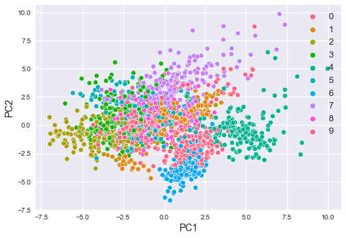
Here, note the following:

we can see that some numbers are well-separated while others are not. For instance, the numbers 2 and 6 are well-separated, while numbers 1 and 8 are not.
observe how most of the numbers are clustered. For instance, all the data points labeled as 6 are grouped into one cluster, and the same can be said for the other digits as well.

This is fascinating because we have managed to represent 64-dimensional data points using only 2-dimensional data points!

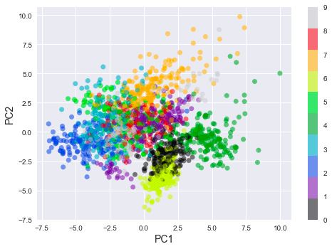
Just as a side note, the book "Python Data Science Handbook"open_in_new uses a colorbar legend instead, which I find to be personally more elegant than the above:


        
        
            
                
                
                    plt.scatter(df['PC1'], df['PC2'],
            c=df['label'], edgecolor='none', alpha=0.5,
            cmap=plt.cm.get_cmap('nipy_spectral', 10))
plt.xlabel('PC1', fontsize=14)
plt.ylabel('PC2', fontsize=14)
plt.colorbar()
plt.show()

This plots the following:

Reconstructing the original images

Recall from the earlier sectionlink that we can reconstruct the original data points using the PCA-transformed points like so:

$$\begin{equation}\label{eq:uZHJ2ib6VdMWoDipSRE} \boldsymbol{Z}=\boldsymbol{X}'\boldsymbol{W}^{T} \end{equation}$$

Where:

$\boldsymbol{Z}$ is the original standardized data points
$\boldsymbol{X}'$ is the transformed data points
$\boldsymbol{W}^T$ is a matrix where the rows are the principal components

Recall that PCA starts off by standardizing the features. Equation \eqref{eq:uZHJ2ib6VdMWoDipSRE} only returns the original standardized features instead of the original features $\boldsymbol{X}$. To recompute the original data points, we must take the inverse of the standardization formula \eqref{eq:vgKhK1G7HFMsCuP90sf}, that is:

$$\begin{equation}\label{eq:Fj8eqYejwXV2HOqpYwg} x^{(i)}_j=z_j^{(i)}\sigma_j+\mu_j \end{equation}$$

Where:

$x_j^{(i)}$ is the $i$-th value of original $j$-th feature
$z_j^{(i)}$ is the standardized value of the $i$-th value in the $j$-th feature
$\sigma_j$ is the standard deviation of the original $j$-th feature
$\mu_j$ is the mean of the original $j$-th feature

Let's use equations \eqref{eq:uZHJ2ib6VdMWoDipSRE} and \eqref{eq:Fj8eqYejwXV2HOqpYwg} to try to reconstruct the original handwritten digits. The idea here is to see how well we can reconstruct the original handwritten digits as we increase the number of principal components.

To set the stage, let's first transform our data points with 64 components and pack the results in a Pandas DataFrame:


        
        
            
                
                
                    sc = StandardScaler()
scaled_X = sc.fit_transform(digits.data)
scaled_X[0]

pca = PCA(n_components=64)
X_pca = pca.fit_transform(scaled_X)
df = pd.DataFrame(X_pca, columns=np.arange(1,65))
df['label'] = digits.target
df.head()
                
            
               1           2         ...   64              label
0  1.914214   -0.954502  ...   8.243855e-15      0
1  0.588980   0.924636   ...   3.086705e-17      1
2  1.302039   -0.317189  ...   2.155553e-17      2
3  -3.020770  -0.868772  ...   1.432069e-17      3
4  4.528949   -1.093480  ...   9.037551e-18      4

Notice how the first two columns are the PC1 and PC2 that we computed in the previous section.

Next, we implement a helper function that computes \eqref{eq:uZHJ2ib6VdMWoDipSRE} and \eqref{eq:Fj8eqYejwXV2HOqpYwg}, and then displays the reconstructed images:


        
        
            
                
                
                    def plot_reconstructed_digits(num_comp=1):
    X_dash = df.iloc[:,:num_comp].to_numpy()
    recovered_standardized = np.dot(X_dash, pca.components_[:num_comp])
    recovered = sc.inverse_transform(recovered_standardized)
    show_digits(recovered)

Note the following:

X_dash is a NumPy array that holds all the values from columns 1 to 64
equation \eqref{eq:uZHJ2ib6VdMWoDipSRE} involves taking the transpose of $\boldsymbol{W}$, but here we do not need to take the transpose of the components because pca.components_ already returns a two-dimensional array with rows as the principal components
the inverse_transform(~) function computes equation \eqref{eq:Fj8eqYejwXV2HOqpYwg}

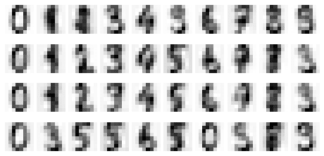
Let's start off by selecting the first 2 components (PC1 and PC2):


        
        
            
                
                
                    plot_reconstructed_digits(2)

This results in the following plot:

Observe how the reconstructed digits are only slightly identifiable. In fact, we can calculate the explained variance ratio to confirm this:


        
        
            
                
                
                    np.sum(pca.explained_variance_ratio_[:2])
                
            
            0.21594970500832741

This means that only 21.6% of the information is preserved when we select just PC1 and PC2. With this limited amount of information preserved, it is not surprising that the reconstructed images are very far from the actual images.

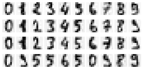
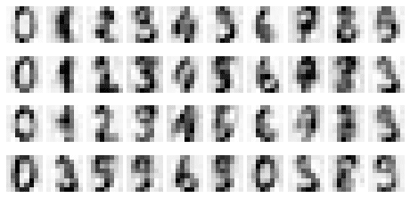
Let's now select 10 components (from PC1 to PC10):


        
        
            
                
                
                    plot_reconstructed_digits(10)

This gives us the following:

This time, we can partially identify the digits. For instance, the number 0 is quite obvious here. The key is that the more components we add, the more information we can preserve, and hence the closer the reconstructed images will be to the actual images.

NOTE

By encoding the images, which were initially represented by 64 features, using only 10 features, we are performing image compression. What's convenient about PCA is that the decoding process of reconstructing the original images (only approximately) is simple and requires only a matrix multiplication and inverse standardization!

Let's compute the explained variance ratio once again:


        
        
            
                
                
                    np.sum(pca.explained_variance_ratio_[:10])
                
            
            0.5887375533730295

By selecting the first 10 components, we can see that we roughly preserve 58.9% of the information contained in the original images!

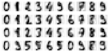
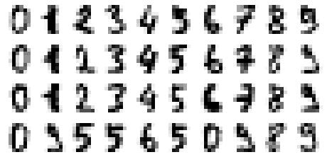
Let's now use 40 components (PC1 to PC40):


        
        
            
                
                
                    plot_reconstructed_digits(40)

This results in the following reconstructed images:

Observe how the digits are very close to the original images! We should therefore expect a very high explained variance ratio:


        
        
            
                
                
                    np.sum(pca.explained_variance_ratio_[:40])
                
            
            0.9507791125066465

This means that by selecting the first 40 principal components, we retain roughly 95% of the original information.

Finally, let's use all 64 principal components. We have already discussed how using all principal components is simply a remapping of the data points into a new coordinate system with the principal components acting as the axes. Since there is no dimensionality reduction, we should be able to reconstruct the original images completely without information loss. Let's confirm this:


        
        
            
                
                
                    plot_reconstructed_digits(64)

This gives us the following reconstructed images:

These are exactly the same sets of images as the actual images! Let's also compute the explained variance ratio when we select all 64 principal components:


        
        
            
                
                
                    np.sum(pca.explained_variance_ratio_[:64])
                
            
            1.0000000000000002

This is to be expected because 100% of the information should be preserved as we're not performing dimensionality reduction here.

NOTE

Notice how the first 2 components explained 21.5% of the original information, and increasing the components to 10 ramped this number up to 58.9%. However, going from the first 40 components to 64 components only yielded a marginal increase of roughly 5% in explainability.

In most cases, the first few components preserve the majority of the information, while the latter components only explain minuscule amounts of information. In other words, there is diminishing returns as we select more principal components. Therefore, when performing dimensionality reduction, we usually select the first few components while discarding the latter components.

Specifying the amount of information to preserve

In the previous example, we have specified the number of components we want like so:


        
        
            
                
                
                    pca = PCA(n_components=64)   # PCA(64)

Instead of specifying the number of components, we can also specify how much information we want to preserve. Sklearn will then select as many components as needed to preserve the specified amount of information.

For example, suppose we wanted to preserve 80% of the original data:


        
        
            
                
                
                    pca = PCA(0.8)   # specify a number between 0 and 1
X_pca = pca.fit_transform(scaled_X)
df = pd.DataFrame(X_pca, columns=np.arange(1,X_pca.shape[1]+1))
df['label'] = digits.target
df.head()
                
            
            
   1          2           ...   21        label
0  1.914214   -0.954502   ...   0.450994    0
1  0.588980   0.924636    ...   0.909818    1
2  1.302039   -0.317189   ...  -0.525917    2
3  -3.020770  -0.868772   ...   0.560421    3
4  4.528949   -1.093480   ...   0.495644    4

We can see that Sklearn has selected 21 components. The sum of explained variance ratio would be around 0.80 as you would expect:


        
        
            
                
                
                    np.sum(pca.explained_variance_ratio_)
                
            
            0.80661732268226

Just to illustrate how the digits look if we keep 80% of the information:


        
        
            
                
                
                    plot_reconstructed_digits(21)

This gives us the following reconstructed plots:

Using PCA to filter out noise

One interesting application of PCA is noise filtering. Recall that PCA works by capturing information in the form of variance while projecting the data points into lower dimensions. The first few principal components capture most of the initial variance (information), while the latter principal components carry much less variance. In other words, most of the important information is captured in the first few principal components, while the latter ones carry more minor and subtle information. Let's understand what this means using an example.

Let's first add some random Gaussian noise to our digits:


        
        
            
                
                
                    np.random.seed(42)
# The value 3 is the standard deviation 
noisy = np.random.normal(digits.data, 3)
show_digits(noisy)

This plots the following:

You can see that the images are now quite noisy compared to the originals shown below:

Let's now use PCA to perform dimensionality reduction, and then reconstruct the original images:


        
        
            
                
                
                    sc = StandardScaler()
scaled_X = sc.fit_transform(noisy)

pca = PCA(0.4)   # Preserve 40% of the information
X_pca = pca.fit_transform(scaled_X)
num_components = X_pca.shape[1]   # 10 components in this case
df = pd.DataFrame(X_pca, columns=np.arange(1,num_components+1))
df['label'] = digits.target

plot_reconstructed_digits(num_components)

This returns the following:

Can you see how the images have much less noise? Even though we can select up to a total of 64 principal components, we only selected the first 10 components. These 10 components capture the most important pieces of information of the original image, which as you would expect, are the digits in black. By discarding the latter components, we effectively eliminate some of the subtle noises.

Using PCA to visualize words

In our Comprehensive Guide on Text Vectorization, we explored several ways we can represent text as numerical vectors. One such technique is called word embedding, in which we encode text as dense vectors that capture the semantics of the word. For instance, similar words such 'hello' and 'hey' are represented as vectors that are positioned near each other, while vectors of unrelated words such as 'hello' and 'car' are far away.

Typically, each word is represented by a vector living in a very high dimension such as $\mathbb{R}^{50}$, which means that we cannot visualize the word embeddings. We can therefore use PCA to reduce the dimension of each word to $\mathbb{R}^2$, and then visually explore the relationship of words.

Firstly, let's import the pre-trained word embedding from a popular natural language processing (NLP) library called genism:


        
        
            
                
                
                    import gensim.downloader as api

model = api.load('glove-wiki-gigaword-50')
model
                
            
            <gensim.models.keyedvectors.KeyedVectors at 0x28e9a86d0>

Here, our model is a word embedding obtained by training a neural network on two large corpora: Wikipedia (as of 2014) and Gigaword, which is the largest corpus of English news documents. The -50 means that each word is represented by a vector of size 50 ($\mathbb{R}^{50}$).

To obtain the vector representation of the word 'hello':


        
        
            
                
                
                    model['hello']
                
            
            array([-0.38497 ,  0.80092 ,  0.064106, -0.28355 , -0.026759, -0.34532 ,
       -0.64253 , -0.11729 , -0.33257 ,  0.55243 , -0.087813,  0.9035  ,
        0.47102 ,  0.56657 ,  0.6985  , -0.35229 , -0.86542 ,  0.90573 ,
        0.03576 , -0.071705, -0.12327 ,  0.54923 ,  0.47005 ,  0.35572 ,
        1.2611  , -0.67581 , -0.94983 ,  0.68666 ,  0.3871  , -1.3492  ,
        0.63512 ,  0.46416 , -0.48814 ,  0.83827 , -0.9246  , -0.33722 ,
        0.53741 , -1.0616  , -0.081403, -0.67111 ,  0.30923 , -0.3923  ,
       -0.55002 , -0.68827 ,  0.58049 , -0.11626 ,  0.013139, -0.57654 ,
        0.048833,  0.67204 ], dtype=float32)

Let's now obtain the vector representation of each word in a list:


        
        
            
                
                
                    tokens = ['hello','goodbye','hey','car','vehicle','python']
word_embeddings = np.array([model[token] for token in tokens])
word_embeddings.shape
                
            
            (6, 50)

Here, word_embeddings is a 2D NumPy array containing the word representations of our 6 words.

Now, let's use PCA to represent each word using just 2 dimensions instead of 50, and then plot the transformed points:


        
        
            
                
                
                    pca = PCA(n_components=2)
result = pca.fit_transform(word_embeddings)
PC1 = result[:, 0]
PC2 = result[:, 1]
plt.figure(figsize=(4.5,4.5))
plt.scatter(PC1, PC2)
plt.xlabel('PC1', fontsize=15)
plt.ylabel('PC2', fontsize=15)
for i, token in enumerate(tokens):
    plt.annotate(token, (PC1[i], PC2[i]), fontsize=15)

This results in the following plot:

Here, you can see that related words such as 'hello', 'goodbye' and 'hey' are clustered, while totally unrelated words such as 'python' are positioned far away. We can therefore conclude that the two principal components do well at preserving the semantics of the words!

Limitations of PCA

Interpreting principal components

PCA reduces the dimensionality of data points by projecting them to lower-dimensional principal components. Although PCA preserves as much information as possible, the principal components contain condensed information that makes them difficult to interpret. For example, consider the previous example of performing dimensionality reduction on the Iris dataset with PCA. Recall that the data points after PCA looked like the following:

We can clearly see that PCA does an excellent job at capturing the essence of the three types of Iris, but the question remains: what do these principal components mean? One way of answering this question is by looking at how the transformation is done:


        
        
            
                
                
                    PC1: 0.52 sepal_length + -0.26 sepal_width + 0.58 petal_length + 0.57 petal_width
PC2: 0.37 sepal_length + 0.93 sepal_width + 0.02 petal_length + 0.07 petal_width

We can see that the value of PC1 is largely affected by the septal length, petal length and petal width, whereas the value of PC2 is dictated by the sepal width. This is as far as we can interpret the principal components; we should be wary of putting labels on PC1 and PC2 because these labels will be based on our own biases and assumptions. By introducing subjectivity into our analysis, our derived insights may be misleading and incorrect.

PCA does not work well for non-linear data points

Consider the following standardized data points:

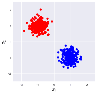
The first principal component in this case is the following green line:

Projecting the data points onto our principal component would result in the following transformation:

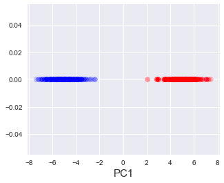
Can you see how the projection does well at capturing information about each cluster? In fact, the explained variance ratio in this case is around 97%!

Now consider the case when we are presented with the following data points:

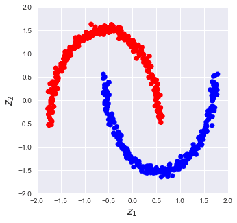
The first principal component in this case would be as follows:

Projecting the data points on this green line would give:

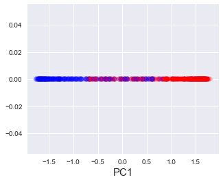
Can you see that, unlike in the previous case, there is no clear separation between the two clusters? In fact, the explained variance ratio in this case is around 72%. This means that simply projecting data points onto a line does not work in cases when the data points are non-linear. To address this issue, there exist other variants of PCA such as kernel PCA or other dimensionality reduction techniques such as auto-encoders that perform non-linear projections. Non-linear projections are obviously beyond the scope of this guide, but if there's demand for such topics, I'm more than happy to write up another comprehensive guide as well!

Selecting the right features for dimensionality reduction

It is tempting to use all the available features for dimensionality reduction such that you preserve as much information as possible of the original dataset. The problem with this is that irrelevant features with high variance would add noise to the resulting principal components, which makes the interpretation even more challenging. The lesson here is therefore to select only the relevant features for dimensionality reduction.

PCA is used only for numerical variables

PCA was designed to work only for numerical variables with the main idea being to preserve the variation of the original data points. Therefore, if we have categorical variables, we must first convert them into numeric variables with techniques such as one-hot encoding. There are similar models to PCA such as multiple correspondence analysis, which are designed to handle categorical variables. For text data, we would normally resort to techniques such as word embedding.

Summary of PCA

PCA is an extremely powerful and popular technique to perform dimensionality reduction. The core idea behind PCA is that information is captured through variance, and the objective is to project data points onto lower dimensions in such a way that minimizes variance loss. The eigenvectors of the variance-covariance matrix represent the principal components, while the corresponding eigenvalues tell us how much information the principal component preserves. In order to select the principal components, we compute a value known as the explained variance ratio of the principal component. The explained variance ratio is the percentage of information that the principal component preserves. In practice, most of the information is captured by the first few principal components.

If you ever want to visualize high-dimensional datasets or feed fewer features into your model, PCA should be your first go-to choice - especially since the implementation is only a few lines of code! Do be cautious of the two limitations of PCA discussed above:

the interpretation of principal components is susceptible to your own biases and assumptions
PCA does not work well for non-linear data points

There are other variations of PCA such as kernel principal component analysis (kernel PCA) that are also worth learning about!

Final words

Thanks for reading this guide, and I hope that you now understand how PCA works - at least at an intuitive level. I know that we glossed over some details, particularly about eigenvectors and eigenvalues, so I'll be writing a separate guide on these topics very soon! Please join our Discord or register an accountopen_in_new to be notified when I publish this guide!

If you're a lecturer at an educational institution, we can offer you a free PDF version of this guide so that you can distribute this guide to your students! Please send us an e-mail over at support@skytowner.com with your .edu e-mail!

Finally, I'm by no means an expert in this subject and so if you found some typos or mistakes, please feel free to let me know either in our Discord or in the comment section below - thanks a lot 🙂.