DBSCAN, or Density-Based Spatial Clustering of Applications with Noise, is a clustering technique that relies on density to group data points. The basic idea behind DBSCAN is that points that are closely packed together belong to the same cluster. DBSCAN is one of the most popular clustering techniques due to its robustness in handling data points of different shapes.

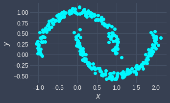
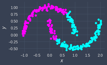
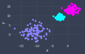
Here's a sneak peek of what DBSCAN can do - given the following input:

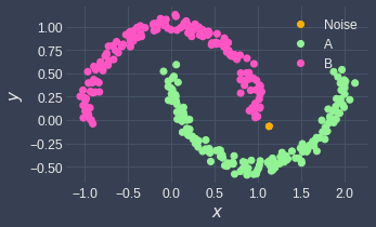
The output of DBSCAN is:

Now, let's get into the details of how DBSCAN works by going over a simple example!

Core, border and noise points

There are 3 types of points that DBSCAN will categorize data points into:

core - a point with at least a pre-defined number of points (minPts) within a pre-defined distance eps
border - a point that is not a core point with at least one core point within the distance eps
noise - a point that is neither core nor border.

After running DBSCAN, we will have the following two pieces of information:

whether each data point is a core, border or noise point.
which cluster each data point belongs to.

In most cases, people care only about the clustering result and ignore output information about the point type (core, border or noise).

Simple example of DBSCAN by hand

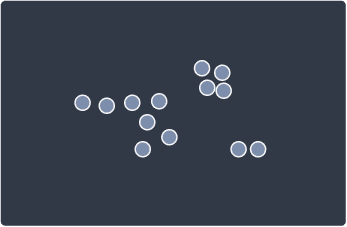
Suppose we are given the following data points on which to perform clustering via DBSCAN:

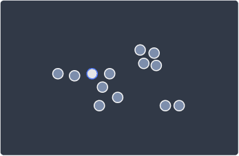
1. Randomly select a data point

The first step is to randomly select a data point:

2. Identify whether the data point is a core or noise point

We then retrieve all points that are within the neighborhood of the point, that is, points that are within the pre-defined distance eps. The type assigned to the data point will depend on the following scenarios:

if the number of neighboring points is equal to or greater than a pre-defined number minPts, then the data point will be considered as a core point and cluster formation begins.
if the number of neighboring points is lower than the minPts, then the data point will be considered as a noise point.

If the data point is identified as a core point, then its neighboring points will be put into the same cluster as that of the data point.

Let us apply this rule to our example:

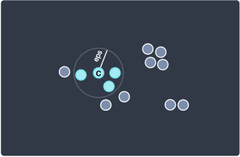
Here, we can see that there are 3 other points in the neighborhood (within distance eps) of the chosen data point. To keep things concrete, let's say that we chose minPts=3, which means that if there are at least 3 neighboring points with a distance less than eps, then the data point will be considered as a core point. In this case, since there are 3 points within the distance of eps, we classify our point as a core point and then proceed with cluster formation. I've added the letter C to make this clear. The 3 neighboring points here will be added to this cluster.

3. Recursively visit each neighboring point and identify whether it is a core or border point

Next, we visit each neighboring point and perform the same neighborhood check and try to identify their type - just as we did for the first data point. The only difference this time is that these neighboring points cannot be, by definition, noise points since they always have a core point within a distance of eps, thereby making them either a border point or a core point.

Back to our example, let's now visit the 3 neighboring points. Drawing three circles will add too much clutter to the diagram, so let's tackle them one by one, starting with the leftmost point:

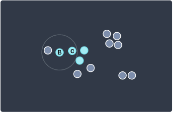
Here, the number of points within the distance of eps is 2, which is lower than minPts=3. This means that this point will be classified as a border point. I've added the letter B to make this clear. The reason why we distinguish border points and core points is that we only add neighboring points to the cluster for core points and proceed to visit those neighbors but we do not do so for border points.

For example, we see that there is a point lying on the left of our current border point. We do not add that point to our cluster nor do we visit that point because the current point is a border point.

Let's now visit the 2nd point at the bottom:

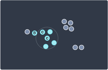
Here, we have a core point because there are 4 neighboring points, which is greater than our minPts=3. Again, since this point is a core point, we will need to visit the two points underneath this point afterward.

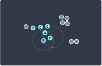
Next, let's visit the 3rd point at the right:

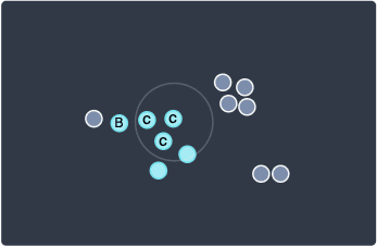
Once again, since there are 3 neighboring points so we classify this point as a core point.

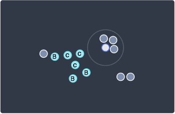
Now, let's get back to the two points at the bottom:

Both these points are border points since they only have one point in their neighborhood.

4. Repeat steps 1 to 3 with a data point that has not yet been visited

We've now exhausted all the points in our first cluster, that is, we have no more points to visit. In such cases, we simply start fresh and randomly visit a data point that has not yet been visited to start forming a new cluster. Let's pick the following point:

I hope you can figure out that these four points will form a cluster with all of them being core points:

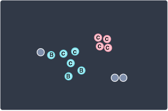
Note that since we've started fresh, these points belong to a new cluster.

We've again run out of points to visit in this cluster, so we randomly pick a point that has not yet been visited:

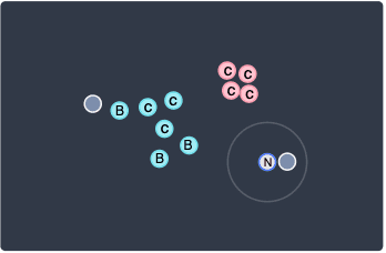
This time, our data point only has one neighboring point. Since 1<minPts, this means that this point is a noise point. I've marked this point as N to denote a noise point. In fact, the point on the right side is also a noise point because of the same reason.

Finally, there is a one last point that we have not visited yet, which is the left-most point:

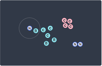
This is once again a noise point.

Final output of DBSCAN

We've now reached the end of the DBSCAN algorithm, and we have:

marked all points as one of core, border or noise
categorized points into different clusters. You can treat noise points as outliers that do not belong to any cluster.

NOTE

Unlike k-means, DBSCAN is a deterministic model. This means that running DBSCAN on the same dataset with the same hyper-parameters will always yield the same results.

Implementing DBSCAN using Python's scikit-learn

Colab Notebook for DBSCAN

Please log in or sign up to access the colab notebook

Click here to access all the Python code snippets (including code to generate the graphs) used for this guide!

lock

Performing clustering using DBSCAN with Python's scikit-learn is easy and can be achieved in a few lines of code! However, the scikit-learn implementation only identifies clusters and noise points - it does not return information about whether a point is a core or border point.

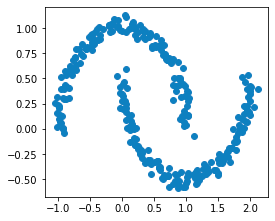
Let's first create a two-dimensional dummy dataset using the make_moons(~) method:


        
        
            
                
                
                    from sklearn.datasets import make_moons
import matplotlib.pyplot as plt

# random_state is for reproducibility
X, y  = make_moons(n_samples=300, noise=0.05, random_state=15)
plt.scatter(X[:,0], X[:,1])
plt.show()

This generates the following plot:

Before we perform DBSCAN, it is good practice to first standardize our data points such that they are on the same scale. This is true for any algorithm that uses distance metrics (e.g. k-means clustering) because the distance metric will be governed by the feature with the highest magnitude. Please refer to this sectionlink of our k-means guide for more details.

We can use scikit-learn's StandardScaler to transform each feature such that it has a mean of 0 and a standard deviation of 1:


        
        
            
                
                
                    from sklearn.preprocessing import StandardScaler

scaler = StandardScaler()
X_scaled = scaler.fit_transform(X)   # X is kept intact!
plt.scatter(X_scaled[:,0], X_scaled[:,1])
plt.plot()

This generates the following plot:

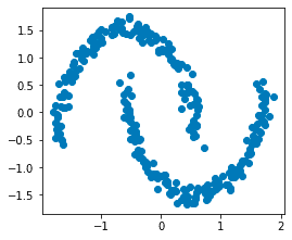
After standardizing our features, the data points should be centered around the origin.

Training a DBSCAN model

We now import the DBSCAN constructor from the sklearn.cluster library. Let's pass the hyper-parameters eps and min_samples into DBSCAN(~) and fit the model:


        
        
            
                
                
                    from sklearn.cluster import DBSCAN
db = DBSCAN(eps=0.25, min_samples=3).fit(X_scaled)

Our DBSCAN model keeps the cluster of each data point in the labels_ property:


        
        
            
                
                
                    # Show the cluster of the first 10 data points
db.labels_[:10]   # Returns a NumPy array
                
            
            array([0, 0, 1, 1, 0, 1, 0, 1, 1, 0])

To see all the different cluster labels, use the set(~) method:


        
        
            
                
                
                    print(f'Clusters: {set(db.labels_)}')
                
            
            Clusters: {0, 1, -1}

We can see that there is a cluster -1, which indicates noise points. We can interpret the noise points as outliers instead of clusters.

To see the total number of points for each cluster, use NumPy's unique(~) method:


        
        
            
                
                
                    import numpy as np
unique, counts = np.unique(db.labels_, return_counts=True)
dict(zip(unique, counts))
                
            
            {-1: 1, 0: 150, 1: 149}

Here, we see that:

there is 1 noise point
there are 150 data points in cluster 0
there are 149 data points in cluster 1

Visualizing clustering results

Finally, let's visualize the clustering results:


        
        
            
                
                
                    from matplotlib.colors import ListedColormap
labels = ['noise', 'A', 'B']
colors = ListedColormap(['black','blue','red'])
scatter = plt.scatter(X_scaled[:,0], X_scaled[:,1], c=db.labels_, cmap=colors)
plt.legend(handles=scatter.legend_elements()[0], labels=labels)
plt.show()

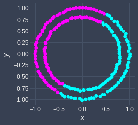
This generates the following plot:

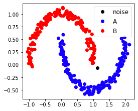
We can see that the noise point as identified by DBSCAN is indeed separated from the red and blue clusters.

WARNING

Unlike k-means, the DBSCAN model does not have a predict(~) method to cluster new unseen data points. This is because of how the two algorithms work. k-means can cluster a new data point by identifying which cluster's centroid is the closest. However, DBSCAN has no notion of centroids and so there is no reliable way to cluster a new data point.

Important properties of DBSCAN

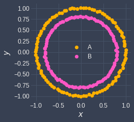
Capable of handling different shapes (vs k-means)

Both k-means and DBSCAN are clustering algorithms, but there are many differences between the two. The major difference is that k-means cannot handle certain shapes such as non-convex and nested circular shapes, whereas DBSCAN is capable of handling these cases:

k-means	DBSCAN

As for why k-means outputs incorrect clustering results, please check out our comprehensive k-means guide.

Robust against outliers

The other major difference is that k-means is heavily affected by outliers, whereas DBSCAN can detect outliers (noise points). If your data has outliers, then consider using DBSCAN.

Highly sensitive to hyper-parameters

DBSCAN's two hyper-parameters eps and minPts describe the density required for cluster formation. DBSCAN's clustering results are highly sensitive to the values of eps and minPts.

For example, setting eps=2 and minPts=3 will result in the following clustering result:

In contrast, setting eps=1 and minPts=3 will generate the following clusters:

There may be sensible choices for eps and minPts in some domains, but we typically have to try out different values to see what works well.

Cannot handle varying densities

Once we set eps and minPts in the beginning, these values remain fixed throughout DBSCAN. This means that DBSCAN cannot handle data points of varying density.

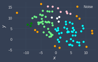
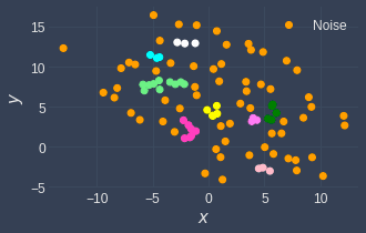
For example, consider the following data points:

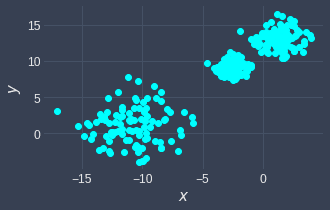
Here, we can see that there are 3 clusters of varying densities. The data points in the bottom left cluster are more spread out compared to the other two clusters.

Let's perform DBSCAN using eps=0.8 and minPts=3:

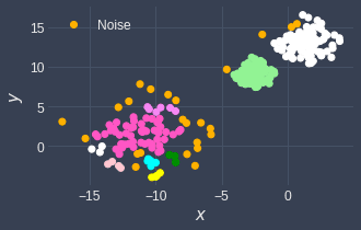
Since we've set a relatively low eps, the data points in the bottom left cluster have become erroneously separated. The potential fix then would be to use a higher eps like 4:

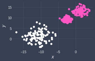
Here, we can see that the bottom left cluster is correct, but since we set the value of eps to be too high, the two clusters on the top have merged together. In this way, DBSCAN cannot handle data points of varying densities.

When we have datasets of varying densities, consider using k-means. For example, the k-means will generate the following clusters for this particular case:

Curse of dimensionality

Similar to k-means, DBSCAN uses a distance metric (typically Euclidean distance) to capture the notion of neighborhood. This poses a problem for high-dimensional data points because the notion of distance breaks down in high dimensions. In fact, regardless of how close or far two data points are, their distance always converges to some constant. Therefore, DBSCAN's clustering result will not be reliable at all for high-dimensional data points.

To avoid the curse of dimensionality, we must reduce the dimensionality of our data points. We can do so by removing or combining features, or by dimensionality reduction techniques such as principal component analysis or auto-encoders.

Closing remarks

DBSCAN is a powerful clustering technique that uses the density of data points to form clusters. The original paper that introduced DBSCAN not only returns clustering results but also identified each data point as border, core and noise point. In practice, only the clustering result is typically of interest.

There are two hyper-parameters for DBSCAN that we must choose before training:

minPts - the minimum number of points for a cluster to be identified as dense
eps (epsilon) - points that are closer than eps will be considered as part of the cluster

There is no single best clustering technique, but I would personally recommend experimenting with both k-means and DBSCAN for every clustering problem because one of them would generally work well.

As always, if you have any questions or feedback, feel free to leave a message in the comment section below. Please join our newsletteropen_in_new for updates on new comprehensive DS/ML guides like this one!

Comprehensive Guide to k-means Clustering

k-means is the most popular unsupervised algorithm whose objective is to cluster data points into a predefined number of clusters, k.

chevron_right

Comprehensive Guide on Hierarchical clustering

The objective of hierarchical clustering is to group data points into nested clusters that can be visualized using a hierarchical tree called the dendrogram.

chevron_right