

Linear regression using Scikit-learn
Start your free 7-days trial now!
This is a tutorial about implementing linear regression using Python's Sciki-learn library. To learn about the theory behind linear regression, check out our tutorial here.
Introduction
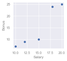
Consider the following dataset about the income of 5 employees:
Salary | Position | Bonus |
|---|---|---|
20 | Manager | 25 |
18 | Manager | 24 |
10 | Staff | 6 |
12 | Staff | 9 |
15 | Staff | 10 |
Here, our goal is to predict the bonus of an employee using their salary and position using linear regression. This means that salary and position are our predictor variables and features, and bonus is our target variable. For linear regression, we should also be mindful about the type of the variables:
salaryis continuouspositionis categorical
Traditionally, linear regression is performed on continuous predictor variables like salary, but the algorithm can be adapted to handle categorical variables as well. To keep things simple, let us first predict the bonus solely based off the salary.
Data visualisation
Here's a quick visualisation of our dataset:
Mathematically, our first goal is to find the optimal weights, $\theta_0$ and $\theta_1$, of a linear curve:
Where,
$y$ is bonus
$x_1$ is salary
$\theta_0$ and $\theta_1$ are the weights (intercept and slope) we wish to optimise
Implementation
Preprocessing
Let's first begin by creating our data-set:
Here, salary and bonus are both a simple 1D Numpy array. However, in order to make them compatible with Scikit-learn's models, we must first convert them to 2D arrays like so:
Similarly, converting our bonus array to a 2D array:
That's it for the preprocessing stage.
Training our model
We can now directly perform linear regression using Scikit-learn:
                    from sklearn.linear_model import LinearRegression
model = LinearRegression()model.fit(x_salary, y_bonus)print("Slope:", model._coef[0])print("Intercept:", model._intercept)


            Slope: 1.9852941176470584Intercept: -14.779411764705877
This means that the equation for the line of best fit is as follows:
Where,
$\hat{y}$ is the predicted
bonusof an employee$x_1$ is the
salaryof an employee
Visualising our model
Since we now have our optimal weights, we can easily graph our linear model:
y_predictions = model.predict(x.reshape(-1,1))
plt.scatter(x_salary, y_bonus)plt.plot(x, y_predictions)plt.xlabel("Salary")plt.ylabel("Bonus")plt.title("Line of best fit - Bonus vs Salary")plt.show()
This produces the following plot:
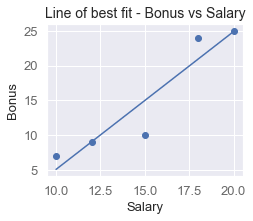
We can see that our model reasonably strikes through the center of our data points.
Performing predictions
To predict employees' bonus given their salary, use the predict(~) method we saw earlier:
The output tells us that:
an employee with
salary=13would have abonusof roughly11.an employee with
salary=16would have abonusof roughly17.
Evaluating performance
Plotting residuals
Residuals tell us how off each of our predictions is, and it is mathematically defined as follows:
Where,
$r^{(i)}$ is the residual of the $i$-th data point
$y^{(i)}$ is the true value of the $i$-th data point
$\hat{y}^{(i)}$ is the predicted value of the $i$-th data point
A high residual for a prediction means that our model did a terrible job at predicting.
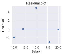
We typically use residual plots to visualise all the residuals:
                    plt.xlabel("Salary", fontsize=13)plt.ylabel("Residual", fontsize=13)plt.title("Residual plot", fontsize=14)
y_predictions = model.predict(x_salary)plt.scatter(x_salary, y_predictions - y_bonus)plt.axhline(0, alpha=0.3)plt.show()
This produces the following:
Mean squared error
Recall from our tutorial covering the theory of linear regression, the mean squared error (MSE) measures how off, on average, our predicted values are:
Where,
$n$ is the size of our dataset ($5$ in this case)
$y^{(i)}$ is the true value of the $i$-th data point
$\hat{y}^{(i)}$ is the predicted value of the $i$-th data point
The MSE comes in handy when you want to compare between different linear regression models. For instance, suppose you fit a polynomial curve instead of a linear curve as we did here, and you want to know which of the two fits the data better. We can compute their respective MSE, and the model with the lower MSE is the one that has the tighter fit.
We can compute the MSE easily using Scikit-learn's built in method:
from sklearn.metrics import mean_squared_error
MSE: 20.8